Hey, welcome to Ask Us Whatever. I’m Joe Sorge.
Well, I thought we’d do things a little differently this time. We’re going to do some garden variety relativity before we go into the studio and work out some math.
So anyway, if you were to read Einstein’s 1905 paper on special relativity, he talks about taking a sphere of energy in the stationary frame and moving it in the moving frame. And he said in the moving frame it will appear like an ellipsoid. And his ellipsoid is oriented vertically, because, I presume, he’s saying that length contraction squishes the sphere in the direction of motion and so you get this vertically oriented ellipsoid.

And then he goes on to start hinting at deriving \(e = mc^2 \). He doesn’t do it in that paper, but it’s on the way.
I don’t believe in length contraction. I’m starting to call it “length contraption” by mistake. But I think that’s accurate, and the reason I think it’s accurate is because he says in that paper that the moving frame will observe this to be an ellipsoid, but he also says people in the moving frame are going to have contracted meter sticks. And if they have contracted meter sticks in the direction of motion, they’re not going to see this as an ellipsoid. They’re going to see it as a sphere, because their meter sticks are going to be contracted in this dimension and then re-expand in that dimension and then re-contract in that dimension.

I think it’s silly. But anyway, it’s the accepted explanation that goes along with the Lorentz transformations in special relativity.
So, in my model, the moving frame would see the sphere, and we’re going to work out some transformations in episodes 7 and 8 to show you how you get a sphere from a stationary frame ellipsoid—and you’re not going to need length contraction to do it. You’re not going to need stretching of space to do it.

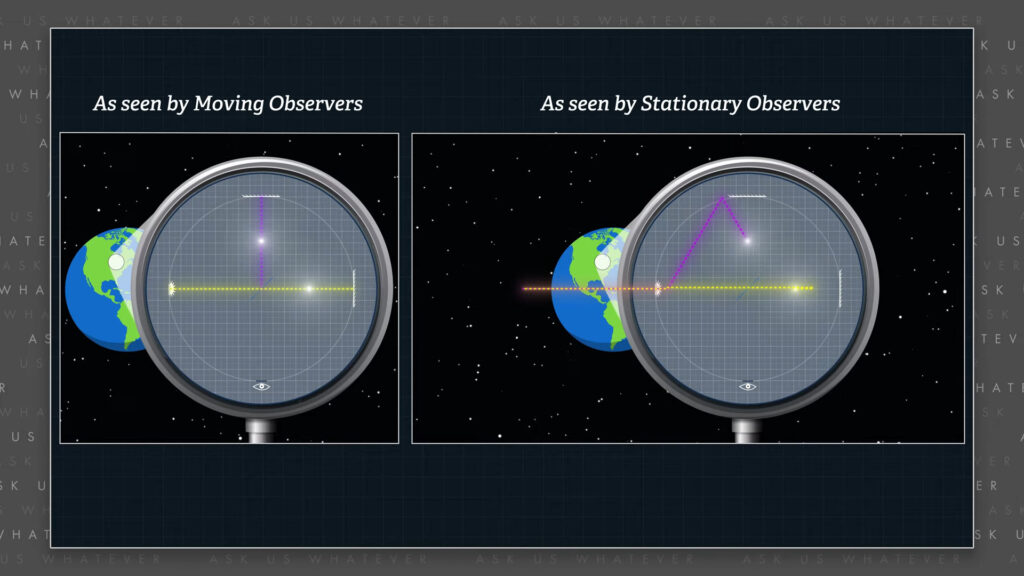
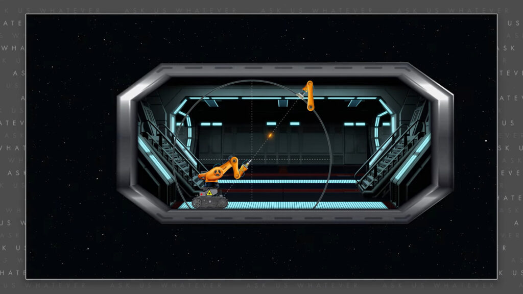
What really happens here is that the light is going faster in the direction of motion and so you get ellipsoidal waves being emitted from a moving source, as seen from the stationary frame.
And so now we’re going to show now we’re going to go into the studio and work out the math to show how we get an ellipsoid and how gamma phi, that I mentioned in the last episode, is going to describe the shape of this ellipsoid.
Ok back from the garden, after a little watermelon break.
Now, in the last episode we began the derivation of the alternative model. And in that derivation, I mentioned that light might travel at gamma-phi times \(c \), but I spent most of the time talking about gamma-\(s \). So now it’s time to derive gamma-phi, and show how it relates to gamma-\(s \). That’s going to take a few steps, and of course some math to show that its logically sound, but hopefully it won’t be too painful.
We need to know how fast light travels if it is emitted at an angle with respect to the direction of motion of the emitter, as viewed from the stationary frame. Let’s call that speed \(c \)-diagonal.
\(c_{diagonal} \)
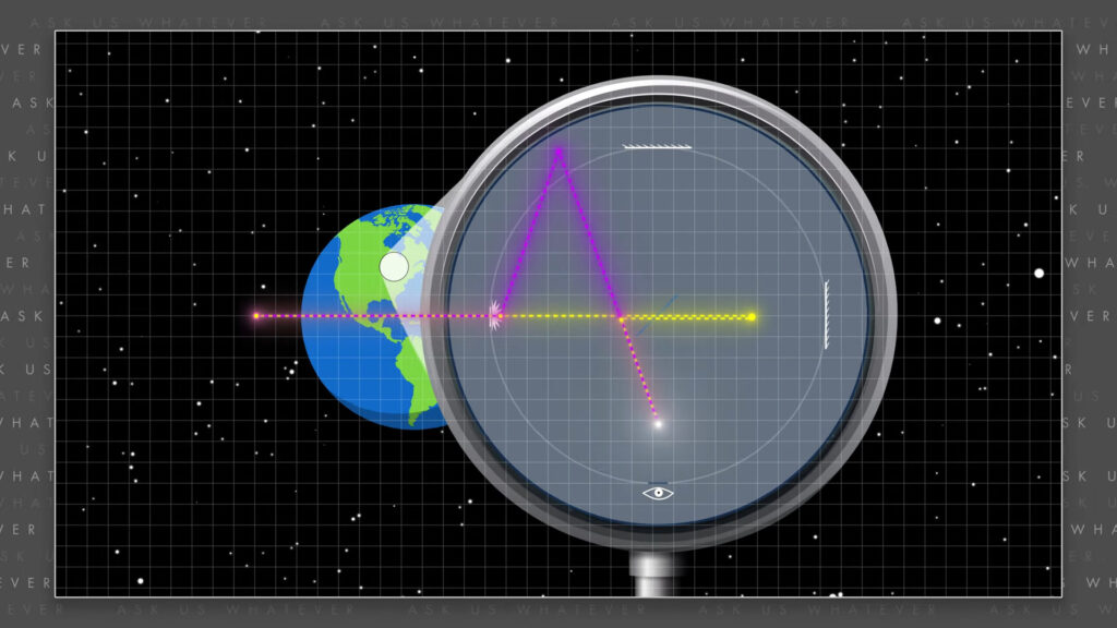
Now, the Michelson Morley experiment required the transverse path of light (in other words the light path that appears to be 90 degrees as seen from the moving frame) to travel at a bit of a diagonal when viewed from the stationary frame.
The time required to travel the diagonal distance is the length of the diagonal path divided by the speed at which light travels along the diagonal path.
\(t_\text{diagonal} = \frac{\sqrt{L’^2 + v^2t^2_\text{diagonal}}}{c_\text{diagonal}} \)
\(L’ \) is the transverse distance as observed from the moving frame and \(v \) is the speed of the IRF (in other words, the speed of Earth in the Michelson Morley experiment).
Squaring both sides,
\(t^2_\text{diagonal} = \frac{(L’^2 + v^2t^2_\text{diagonal})}{c^2_\text{diagonal}} \)
and after rearranging, we see that,
\(t_\text{diagonal, round trip} = 2\frac{L’}{\sqrt{c^2_\text{diagonal} \space – \space v^2}} \)
the round trip diagonal travel time equals two times the transverse path length \(L’ \) divided by the square root of diagonal light speed squared minus the speed of the IRF squared.
This expression would be consistent with special relativity if the \(c \)-diagonal term is simply equal to speed \(c \). But our alternative model provides for the possibility of speeds other than \(c \), so let’s continue and solve for \(c \)-diagonal.
To be consistent with the Michelson Morley result, we will equate the round trip diagonal travel time with the round trip longitudinal travel time, as derived in the prior episode. And after some fast algebra using the square root of 1 plus \(v \)-squared over \(c \)-squared for gamma-\(s \), [ok you can pause the video here]
\(\frac{2L’}{\sqrt{c^2_\text{diagonal} \space – \space v^2}} = \frac{2L’ \gamma_s c}{\gamma^2_s c^2 – v^2} \)
\(\frac{1}{\sqrt{c^2_\text{diagonal}} \space – \space v^2} = \frac{\gamma_s c}{c^2 + v^2 – v^2} = \frac{\gamma_s}{c} \)
\(\frac{1}{c^2_\text{diagonal} \space – \space v^2} = \frac{\gamma^2_s}{c^2} \)
\(\frac{c^2}{\gamma^2_s} + v^2 = c^2_\text{diagonal} \)
\(\frac{c^2}{1 + \frac{v^2}{c^2}} + v^2 = c^2_\text{diagonal} \)
\(\frac{c^2 + v^2 + v^4/c^2}{1 + \frac{v^2}{c^2}} = c^2_\text{diagonal} \)
\(c^2 \frac{1 + \frac{v^2}{c^2} + \frac{v^4}{c^4}}{1 + \frac{v^2}{c^2}} = c^2_\text{diagonal} \)
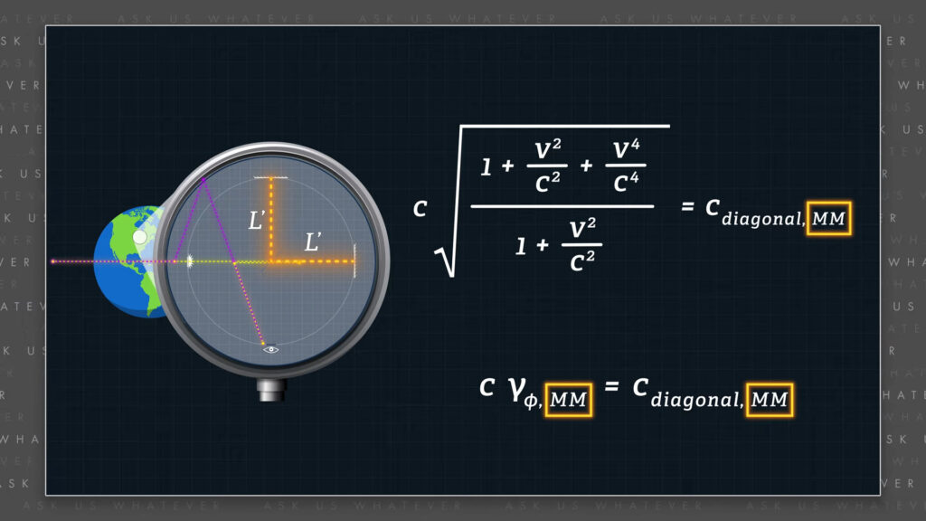
\(c \sqrt{\frac{1 + \frac{v^2}{c^2} + \frac{v^4}{c^4}}{1 + \frac{v^2}{c^2}}} = c_\text{diagonal} \)
we see that diagonal light speed is a multiple of the constant \(c \). We call the square root term gamma-phi for Michelson Morley setups, and we represent diagonal light speed as gamma-phi MM times \(c \).
\(c_\text{diagonal, MM} = \gamma_{\phi , MM} c \)
We use the symbol “MM” to note that this formula is specific to a Michelson Morley type of setup. We will derive a more general formula for gamma-phi later in this episode.
If we call the ratio of \(v \) divided by \(c \), beta
\(\beta = v/c \)
then gamma-phi can be written as,
\(\gamma_{\phi, MM} = \sqrt{\frac{1 + \frac{v^2}{c^2} + \frac{v^4}{c^4}}{1 + \frac{v^2}{c^2}}} = \)
\(\sqrt{\frac{1 + \beta^2 + \beta^4}{1 + \beta^2}} = \)
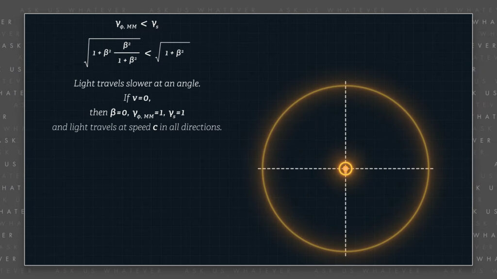
\(\sqrt{1 + \beta^2 \frac{\beta^2}{1 + \beta^2}} < \sqrt{1 + \beta^2} = \gamma_s \)
The square root of 1 plus beta-squared plus beta to the fourth all divided by 1 plus beta-squared.
Note that gamma-phi is less than gamma-\(s \), except for longitudinal motion. In other words, light travels less quickly when traveling at an angle with respect to the direction of IRF motion. If the IRF is stationary, \(\beta = 0 \), and so \(\gamma_\phi = 1 \), and \(\gamma_s = 1 \) and light travels at speed \(c \) in all directions. In other words, light speed is isotropic when the source of the light is stationary
It’s now possible to confirm that the time required for light to travel diagonally in a Michelson Morley setup as observed from the stationary frame is \(\gamma_s \) times \(L’/c \). In other words, to confirm that in the alternative model, time is dilated according to the factor gamma-\(s \). OK here’s some fast algebra, and you can pause the video to examine it carefully.
\(t_\text{diagonal} = \frac{\text{diagonal distance}}{c_{diagonal}} = \)
\(\frac{\sqrt{L’^2 + v^2 t^2_\text{diagonal}}}{\gamma_\phi c} \)
\(t_\text{diagonal} = \frac{\sqrt{L’^2 + v^2 t^2_\text{diagonal}}}{\sqrt{\frac{1 + \beta^2 + \beta^4}{1 + \beta^2}}c} \)
\(\sqrt{\frac{1 + \beta^2 + \beta^4}{1 + \beta^2}}ct_\text{diagonal} = \)
\(\sqrt{L’^2 + v^2 t^2_\text{diagonal}} \)
\((\frac{1 + \beta^2 + \beta^4}{1 + \beta^2})c^2 t^2_\text{diagonal} = \)
\(L’^2 + v^2 t^2_\text{diagonal} \)
\(t^2_\text{diagonal} = \frac{L’^2}{(\frac{1 + \beta^2 + \beta^4}{1 + \beta^2})c^2 – v^2} \)
\(t^2_\text{diagonal} = \frac{L’^2}{\frac{c^2}{1 + \frac{v^2}{c^2}}} = \frac{\gamma^2_s L’^2}{c^2} \)
\(t_\text{diagonal} = \frac{\gamma_s L’}{c} = \gamma_s t’ \)
We see that the time for light to travel diagonally as observed from the stationary frame is gamma-\(s \) times \(t’ \). This is consistent with our assumption that time dilation between stationary and moving frames is proportional to gamma-\(s \).
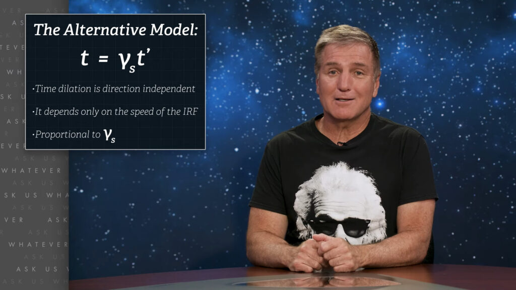
\(t = \gamma_s t’ \)
Now that’s a very important point. Time dilation is direction-independent. It depends only on the speed of the reference frame.
Einstein believed time dilation was proportional to the Lorentz gamma factor. I’m saying time dilation is proportional to gamma-\(s \), which if you recall from the prior episode is essentially numerically equivalent to the Lorentz gamma factor at speeds at which satellites and planets travel, down to fifteen digits. In other words, tests of time dilation carried out to date have not differentiated gamma-\(s \) from the Lorentz gamma factor. Hopefully someone will lend me a couple of satellites so we can do a more precise experiment.
Now, the formula for gamma-phi above is appropriate for a Michelson Morley experiment where the angle phi is determined by the velocity \(v \) of the IRF relative to the stationary frame. However, light can be emitted from a moving source at any angle. So let’s derive a more general formula for gamma-phi as a function of the emission angle.


If we replace \(t \)-diagonal with gamma-\(s \) times \(t’ \) in one of the equations from above,
\((\frac{1 + \beta^2 + \beta^4}{1 + \beta^2})c^2 t^2_\text{diagonal} = \)
\(L’^2 + v^2 t^2_\text{diagonal} \)
\((\frac{1 + \beta^2 + \beta^4}{1 + \beta^2})c^2 \gamma^2_s t’^2_\text{diagonal} = \)
\(L’^2 + v^2 \gamma^2_s t’^2_\text{diagonal} \)
And then divide both sides by \(c\)-squared times gamma-\(s \)-squared times \(t’ \)-diagonal squared,
\(\gamma^2_{\phi, MM} = (\frac{1 + \beta^2 + \beta^4}{1 + \beta^2}) = \)
\(L’^2 + v^2 \gamma^2_s t’^2_\text{diagonal} \)
we see that gamma-phi-MM-squared is equal to \(L’ \)-squared divided by \(c \)-squared times gamma-\(s \)-squared times \(t’ \)-diagaonal squared plus \(v \)-squared over \(c \)-squared. And since \(L’ \) divided by \(c \) is equal to \(t’ \), which is also equal to \(t’ \)-diagonal, we find that
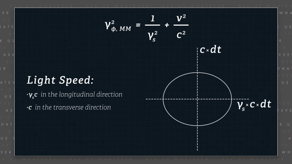
\(\gamma^2_{\phi, MM} = \frac{1}{\gamma^2_s} + \frac{v^2}{c^2} \)
gamma-phi-MM-squared is equal to 1 over gamma-\(s \)-squared plus \(v \)-squared over \(c \)-squared, which is in the form of an equation for an ellipse. And since we learned in Episode 6.1 that light travels at gamma-\(s \) times \(c \) in the longitudinal direction and speed \(c \) in the transverse direction, we can check to see if light waves coming from a moving source radiate in the shape of an ellipsoid with major axis equal to gamma-\(s \) times \(c \) times \(dt \), and minor axes equal to \(c \) times \(dt \).
And in polar coordinates, the radius of an ellipse can be computed with,
\(r_\text{ellipse} = \frac{ab}{\sqrt{a^2 \sin^2 \phi + b^2 \cos^2 \phi}} \)
\(a \) times \(b \) divided by the square root of \(a \)-squared times the sine squared of phi plus \(b \)-squared times the cosine squared of phi; where \(a \) represents the major axis, which here would be gamma-\(s \) \(cdt \), and \(b \) represents the minor axis, which here would be \(cdt \). This produces the following equation.
\(r_\text{ellipse} = \frac{\gamma_s cdtcdt}{\sqrt{(\gamma_s cdt)^2 \sin^2 \phi + (cdt)^2 \cos^2 \phi}} \)
Factoring \(cdt \) from the numerator and denominator,
\(r_\text{ellipse} = \frac{\gamma_s}{\sqrt{\gamma^2_s \sin^2 \phi + \cos^2 \phi}}cdt = \)
\(\frac{\sqrt{1 + v^2/c^2}}{\sqrt{1 + v^2 \sin^2 \phi / c^2}}cdt \)
we see that the radius of light emitted from a moving source is equal to gamma-\(s \) divided by the square root of 1 plus \(v \)-squared over \(c \)-squared times the sine squared of phi, all multiplied by \(c \) times \(dt \).
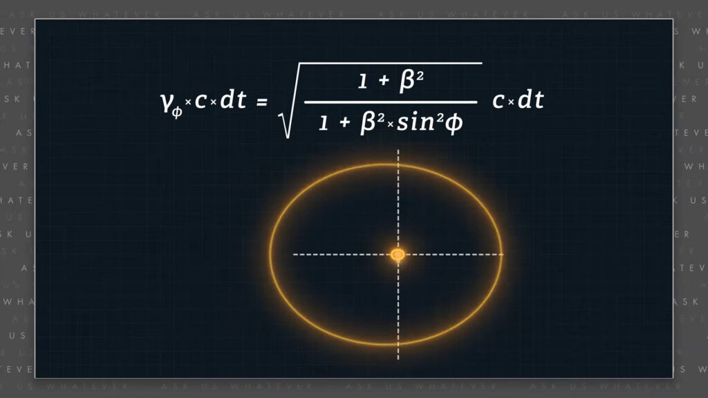
In general, the wave pattern of light coming from a moving source is in the shape of an ellipsoid described in two dimensions by the following formula,
\(\gamma_\phi cdt = \sqrt{\frac{1 + \beta^2}{1 + \beta^2 \sin^2 \phi}}cdt \)
where phi is the angle between the direction of the moving source and the direction of light emitted from the source, as measured from the perspective of stationary frame observers. Therefore a more general formula for gamma-phi at any angle is,
\(\gamma_\phi = \sqrt{\frac{1 + \beta^2}{1 + \beta^2 \sin^2 \phi}} \)
the square root of 1 plus beta squared divided by 1 plus beta squared times the sine squared of phi.
For any given value of \(v \), light travels at its greatest speed in the longitudinal direction. When the \(\sin \phi \) is 1 light travels at speed \(c \) in the transverse direction. That is, light emitted transversely from a moving source travels at speed \(c \), where the angle of emission is measured from the stationary frame. Again, light travels at speed gamma-\(s \) times \(c \) when emitted in the direction of reference frame motion and at speed \(c \) when emitted at right angles to reference frame motion.
If we compare the angular formula for gamma-phi with the formula derived from the Michelson Morley experiment,
\(\gamma_\phi = \sqrt{\frac{1 + \beta^2 + \beta^4}{1 + \beta^2}} = \sqrt{\frac{1 + \beta^2}{1 + \beta^2 \sin^2 \phi}} \)
we find that they are equal when phi is the angle,
\(\phi = arccos (\frac{v}{c_\text{diagonal}}) \)
as seen from the stationary frame, at which light must travel to strike the mirror along the path that appears to be transverse in the moving frame, confirming that light, in the alternative model, radiates in an elliptical pattern from a moving source, as observed from the stationary frame.
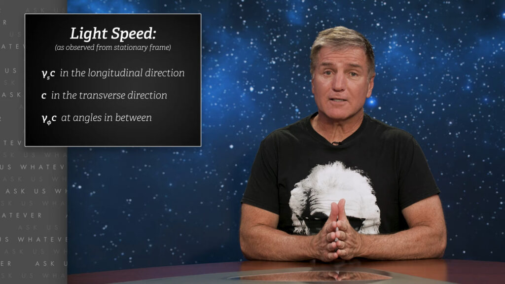
Let’s summarize here. When we eliminate length contraction from the Lorentz/Einstein model, it draws us to the possibility that light travels at speed gamma-\(s \) times \(c \) in the longitudinal direction when emitted from a moving source, and at speed \(c \) in the transverse direction – and somewhere in between when traveling at an angle.
We will show in the next few episodes that observers in the moving frame will still observe light to travel at speed \(c \) in their frame of reference in all directions when coming from a source traveling with them in their frame. In other words, where gamma-phi is equal to 1. So our model is consistent with our Earth-bound observations that light travels at speed \(c \).
And although I didn’t say it explicitly, the alternative model implies a preferred frame of reference. We will cover more in future episodes, but the alternative model challenges special relativity’s postulate that all relativity is symmetric.
Alright, that’s it for now. In the next few episodes, we will derive the Lorentz distance and time transformations for both special relativity and the alternative model. If you have any questions, please write them in the comments section. I’m Joe Sorge, and thanks for watching.