You’re most likely watching this video using a connection to the internet; which at some point typically involves the transmission of light signals through fiberoptic cables.
How fast do you think those light signals travel? It’s not at speed c. Fiberoptic cables are typically filled with glass, which slows light to about two-thirds of its speed through vacuum. So why do you think this happens? What’s the reason for the slowing of light at the molecular or atomic level?
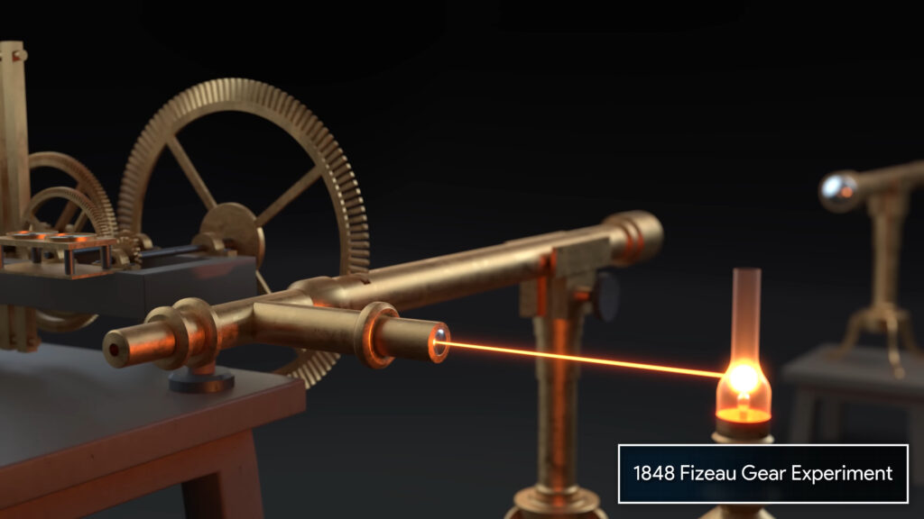
A careful look at the results produced by the 1859 Fizeau and 1913 Sagnac experiments will help us understand why light travels more slowly through refractive media, and will shed light on a possible molecular mechanism for the slowing.
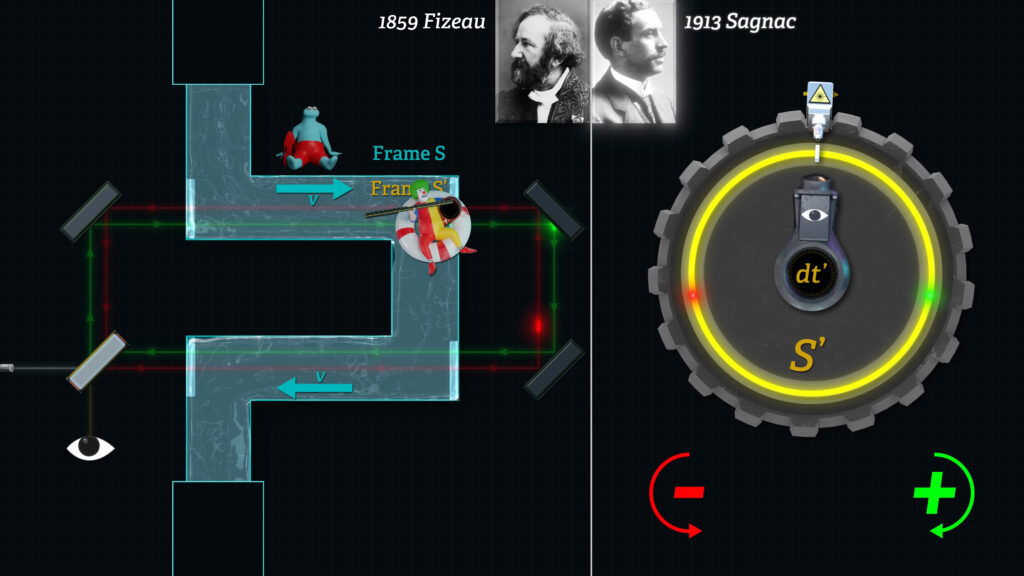
Both the Sagnac and Fizeau setups measure the time required for light to travel either “downstream” or “upstream” through a moving substance, like water. If the travel times are different in the two directions, the devices reveal a shift in a wave interference pattern.
The mystery that we need to solve, and what is going to reveal the mechanism behind the slowing of overall light speed, is why a Sagnac interference shift does not change, whether light passes through vacuum or through a refractive medium.
Whereas in a Fizeau device, the nature and the motion of the refractive media affects the amount by which the interference fringes shift.
The difference in those outcomes speaks directly to the key question of whether light truly slows down to a new, constant velocity through the entirety of a refractive substance, or whether it travels at its normal vacuum speed in between refractive molecules, but travels more slowly when hindered by those refractive molecules.
Let’s develop a model that’s consistent with Special Relativity, for now, to help us understand the underlying concepts.
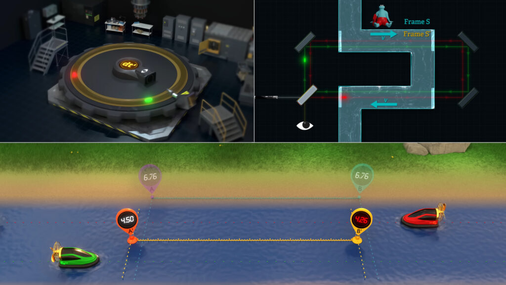
Consider a hovercraft that is elevated by a powerful air cushion above a river of water.
Let’s assume for now that the craft gets all of its horizontal speed from a propeller fan and that the river does not drag it downstream. If the hovercraft’s propeller fan were to be turned off, it will hover above the moving water and remain stationary with respect to the land. But when the hovercraft’s engines are set to full speed, the hovercraft will have a speed of c-sub-h (\(c_h \)) relative to the land.
𝑣=𝑠𝑝𝑒𝑒𝑑 𝑜𝑓 𝑟𝑖𝑣𝑒𝑟 “𝑓𝑟𝑎𝑚𝑒” 𝑟𝑒𝑙𝑎𝑡𝑖𝑣𝑒 𝑡𝑜 𝑙𝑎𝑛𝑑
\(𝑐_ℎ \)=𝑠𝑝𝑒𝑒𝑑 𝑜𝑓 ℎ𝑜𝑣𝑒𝑟𝑐𝑟𝑎𝑓𝑡 𝑟𝑒𝑙𝑎𝑡𝑖𝑣𝑒 𝑡𝑜 𝑡ℎ𝑒 𝑙𝑎𝑛𝑑
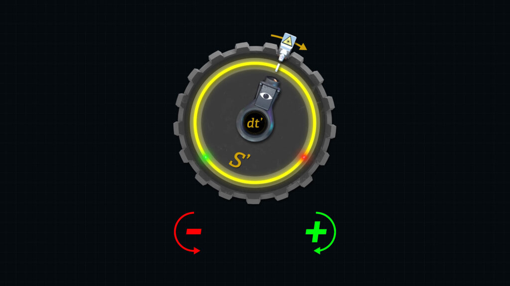
The hovercraft in our model represents a light signal. And the river represents a moving reference frame. Don’t worry about the composition of the river for now. Our imaginary river does not alter the speed of the hovercraft. The river is simply a reference frame that we will call Frame S’. The river is moving at speed v with respect to the banks of the river, which we will call Frame S.
We can measure the hovercraft’s travel time in several ways. One-way is relative to the distance markers on the shore.
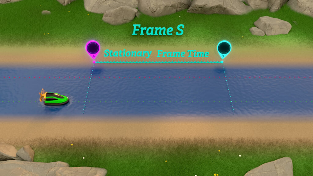
The time required to travel between markers on the shore is what we will call stationary frame time; it will be measured with clocks on the shore.
We will keep track of stationary frame time with the symbol t, and the difference in stationary times with the symbol dt.
We can also measure the hovercraft’s travel time relative to markers floating with the current of the river.
We will call the time required for the hovercraft to travel from one floating marker to another floating marker, time dt’.
To make sure that our model will be compliant with Special Relativity, time dt’ will be measured with clocks floating with the river.
The time required for the hovercraft to pass two floating markers 100 meters apart will be different than the time required for the hovercraft to pass two land-based markers 100 meters apart; and the difference in these two times will also depend on whether the hovercraft is traveling downstream or upstream, and also on the method used to synchronize clocks A, A’, B, and B’.
In Episode 9.5.A we illustrated how Einstein’s method of clock synchronization causes Clocks A’ and B’ to report different times of day. And this can influence the measurement of elapsed time.
Now, in order to keep track of distance measurements, we can symbolize distance traveled relative to markers on the land as dx.
𝑑𝑥 = 𝑑𝑖𝑠𝑡𝑎𝑛𝑐𝑒 𝑡𝑟𝑎𝑣𝑒𝑙𝑒𝑑 𝑚𝑒𝑎𝑠𝑢𝑟𝑒𝑑 𝑤𝑖𝑡ℎ 𝑙𝑎𝑛𝑑 𝑚𝑎𝑟𝑘𝑒𝑟𝑠
Similarly, we can symbolize distances traveled relative to markers floating on the river as dx’. Keep in mind that in Special Relativity moving frame distances are measured with contracted meters’.
𝑑𝑥′ = 𝑑𝑖𝑠𝑡𝑎𝑛𝑐𝑒 𝑡𝑟𝑎𝑣𝑒𝑙𝑒𝑑 𝑚𝑒𝑎𝑠𝑢𝑟𝑒𝑑 𝑤𝑖𝑡ℎ 𝑚𝑎𝑟𝑘𝑒𝑟𝑠 𝑓𝑙𝑜𝑎𝑡𝑖𝑛𝑔 𝑜𝑛 𝑡ℎ𝑒 𝑟𝑖𝑣𝑒𝑟
Now, Einstein developed Special Relativity using inertial reference frames, meaning systems moving in straight lines at constant velocity, just like the linear river in our model. But Fizeau and Sagnac created experimental setups in which the light signal traveled over a closed loop path. In other words, the light signals returned to their point of origin.
In both the Fizeau and Sagnac experiments, the light signals travel from the beam splitter, around a loop that may contain a refractive medium, and back to the same beam splitter where they recombine.
In a Fizeau setup, the light path and the beam splitter do not move relative to the laboratory. Which means that both light signals travel the same distance, dx, relative to the laboratory in both directions. But the distances the light signals travel with respect to Fizeau’s moving water, dx’, will depend on the speed of Fizeau’s moving water and the direction of the light signal.
In other words, if there were distance markers floating in Fizeau’s moving water, distances measured using those floating markers would not be equal to distances measured using markers that are stationary in the laboratory. In mathematical terms, dx will not be equal to dx’ when Fizeau’s water is moving.
\(dx≠dx’ \), when \(v>0 \)
In a Sagnac setup, the beam splitter and the light path (a fiber optic cable, or an array of mirrors) both move relative to the laboratory. The distances the two light signals travel from beam splitter, around the loop, and back to the beam splitter will be the same in the moving frame of the beam splitter. It’s very important to understand this.
If we had an observer who was moving with the setup, that observer would measure light to travel the same distance dx’ in either direction. But the distance the light signals travel with respect to the laboratory, dx, will depend on the speed of the rotating device.
The important difference between either a Sagnac or a Fizeau setup, and a Special Relativity setup, is that Special Relativity measures the speeds of things moving in straight lines using more than one clock.
There is a clock at the starting point and a different clock at the finish line. And as I showed in Episode 9.5.A, we cannot trust these to report the same time of day when the clocks have been synchronized using Einstein’s clock synchronization method.
But in a Sagnac or Fizeau experiment, the travel-path forms a closed loop, and the same clock is used to measure time at the start and at the finish. This takes away any concern about the method used for clock synchronization. There’s only one clock, and so we need not worry about clocks reporting different times at different locations.
So, in order to explain how the Sagnac and Fizeau experiments work at the molecular level, we will take our linear river model and make it into a circular, lazy river.
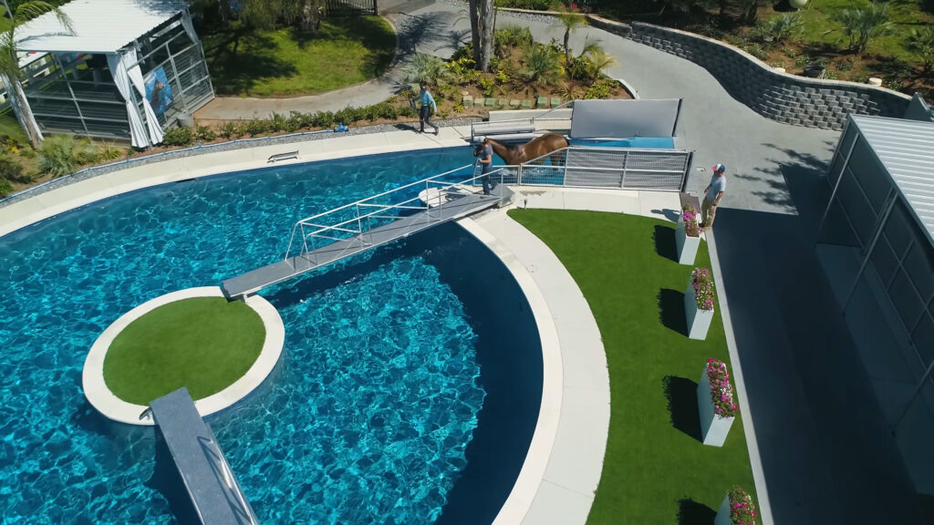
To bring some reality to this, we searched for real hovercraft traveling in circles over a lazy river, but obviously couldn’t find one. However, we did find this circular swimming pool for rehabilitating injured horses, and we just had to show it to you because it’s so cool. Nevertheless, to keep our analogy precise we will stick with our animated model of hovercraft navigating a circular river.
It’s important to note that in our lazy river model, there will be only one stationary-frame clock, attached to a single, land-based distance marker. This is analogous to the single beam splitter in the Fizeau setup.
And there will be only one moving-frame clock, floating around the lazy river attached to a single, floating distance marker. This is analogous to the moving beam splitter in a Sagnac setup.
Next, we need to talk about our analogy for the refractive index in the Fizeau and Sagnac experiments. We assume that an uncluttered river has a refractive index of 1, meaning that a hovercraft will move at its normal speed with respect to the stationary and floating markers respectively. This is analogous to light travelling through vacuum.
But if there are large logs floating in the river, they will increase the “refractive index for hovercraft” to a value greater than 1. In other words, it will take longer for a hovercraft to travel over a river cluttered with obstructing logs, since there will be a delay associated with the hovercraft navigating around each log. We can think of molecules that refract light as obstructing logs, creating temporary barriers to the passage of light through what otherwise would be vacuum.

I’m not necessarily saying that photons are solid particles that bounce into solid molecular objects – it’s obviously more complicated than that. But you will soon see that the substance of the refractive medium causes a delay in the normal transmission of light signals along the light path.
If a refractive medium is stationary relative to the laboratory – in other words the speed of Frame S’, v, is zero – a light signal will travel at about n times slower than if there were no refractive molecules present.
Light passing through a stationary refractive medium is analogous to the hovercraft navigating through a sea of logs floating on a stationary lazy river.
The hovercraft will attempt to travel at its speed c-sub-h (\(𝑐_ℎ \)) between logs, but will be delayed with each log encountered.
In a Sagnac setup, the refractive medium, if any, moves together with the light path relative to the stationary frame. The light path can be a series of mirrors in a vacuum chamber or in air, or a fiberoptic cable filled with glass.
The important point is that in a Sagnac setup we measure the progress of two counterpropagating light signals using the beam splitter which acts both as a moving distance marker and a clock.
In the original Sagnac experiment, dx’ was the distance from the beam splitter, around the light circuit, and back to the beam splitter. In our lazy river analogy, this would be the distance that an observer floating along the river would observe a hovercraft to travel if the observer used only the distance markers floating on the river. In a Sagnac setup, this dx’ distance is constant, regardless of how fast the apparatus (or the river) moves with respect to the laboratory (or the land).
𝑓𝑟𝑎𝑚𝑒 𝑆 𝑚𝑎𝑟𝑘𝑒𝑟𝑠 ≡ 𝑙𝑎𝑏𝑜𝑟𝑎𝑡𝑜𝑟𝑦 𝑚𝑎𝑟𝑘𝑒𝑟𝑠≡𝑙𝑎𝑛𝑑 𝑚𝑎𝑟𝑘𝑒𝑟𝑠
𝑓𝑟𝑎𝑚𝑒 𝑆′ 𝑚𝑎𝑟𝑘𝑒𝑟𝑠 ≡ 𝑚𝑜𝑣𝑖𝑛𝑔 𝑙𝑖𝑔ℎ𝑡 𝑝𝑎𝑡ℎ 𝑚𝑎𝑟𝑘𝑒𝑟𝑠≡𝑓𝑙𝑜𝑎𝑡𝑖𝑛𝑔 𝑟𝑖𝑣𝑒𝑟 𝑚𝑎𝑟𝑘𝑒𝑟𝑠
𝑆𝑎𝑔𝑛𝑎𝑐 𝑠𝑒𝑡𝑢𝑝 ≡ 𝑑𝑥′𝑐𝑜𝑛𝑠𝑡𝑎𝑛𝑡, 𝑑𝑥 𝑣𝑎𝑟𝑖𝑎𝑏𝑙𝑒
In either a Sagnac or a Fizeau experiment, we would like to determine what effect the speed of Frame S’ has on the time measurements for light to complete the counterpropagating trips in the positive (or downstream) versus the negative (or upstream) directions.
Since dx’ is constant in a Sagnac experiment, we would like to express elapsed time, dt-sub-n-plus-or-minus (\(𝑑𝑡_{𝑛±} \)), in terms of dx’, n, v, and c. We defined the meanings of these terms in Episode 9.5.A.
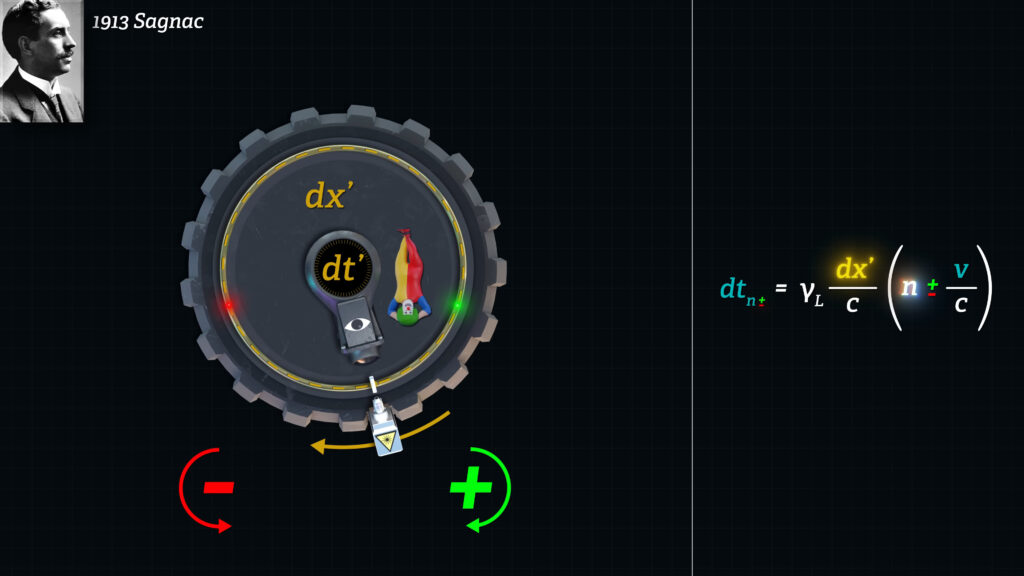
We can use the time formula that we derived in Episode 9.5.A to compute this time.
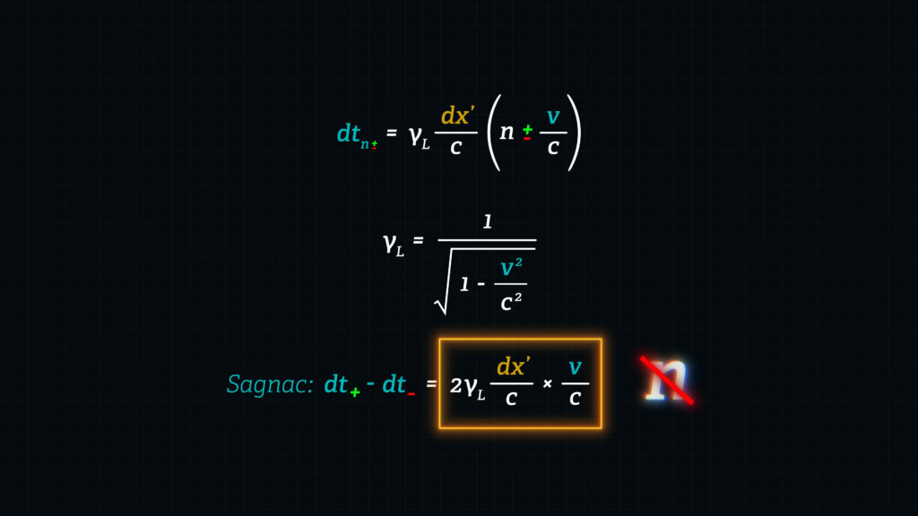
\(𝑑𝑡_{𝑛±} = 𝛾𝐿 \frac{𝑑𝑥′}{𝑐} (𝑛 ± \frac{𝑣}{𝑐}) \)
Dt-sub-n-plus-or-minus is the time for light (or a hovercraft) to travel in either the plus (downstream) or minus (upstream) directions starting at a moving clock and traveling around the circuit back to the same moving clock, as converted to stationary frame units of time: that is, denominated in stationary seconds. Based on the time dilation concept of Special Relativity, the gamma(L) factor converts moving clock time, denominated in seconds-prime, to stationary clock time, denominated in seconds. You’ll recall that moving clocks tick gamma(L) times slower than stationary clocks.
Gamma(L) times dx’ over c is the average Frame S time required for two light signals to each travel distance dx’ at speed c.
\(𝛾𝐿 \frac{𝑑𝑥′}{𝑐} = \) 𝑠𝑖𝑚𝑝𝑙𝑒 𝑎𝑣𝑒𝑟𝑎𝑔𝑒 𝑜𝑓 + 𝑎𝑛𝑑 − 𝑓𝑟𝑎𝑚𝑒 𝑆 𝑒𝑙𝑎𝑝𝑠𝑒𝑑 𝑡𝑖𝑚𝑒𝑠 𝑡𝑜 𝑡𝑟𝑎𝑣𝑒𝑙 𝑑𝑥′
\(𝑑𝑡_{𝑛±} = 𝛾𝐿 \frac{𝑑𝑥′}{𝑐} ( 𝑛 ± \frac{𝑣}{𝑐}) \)
In our hovercraft analogy,
\(𝑑𝑡_{𝑛±} = 𝛾𝐿 \frac{𝑑𝑥′}{𝑐_ℎ} (𝑛 ± \frac{𝑣}{𝑐_ℎ}) \)
if there are obstructing logs floating on the river, they will slow down the craft and the time for the hovercraft to travel the same distance over the river will increase by a factor of n.
The v divided by c-sub-h term reflects the differential time required to travel the distance between moving markers.
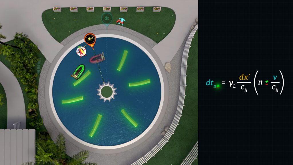
For example, if the hovercraft is headed downstream, the time required to travel between two moving logs will be affected by the speed of the river. Recall that the speed of the hovercraft is constant with respect to the land, but if the logs are moving downstream with respect to the land, the hovercraft will need to “catch up with” the receding logs, and vice versa for the hovercraft heading upstream.
Note that in the lazy river analogy, the c terms in the denominators of the dt-sub-n-plus-or-minus (\(𝑑𝑡_{𝑛±} \)) formula will be the speed c-sub-h (\(𝑐_ℎ \)) of the hovercraft with respect to the land.
\(𝑑𝑡_{𝑛±} = 𝛾𝐿 \frac{𝑑𝑥′}{𝑐_ℎ} (𝑛 ± \frac{𝑣}{𝑐_ℎ}) \)
And so, the extra distance and extra time required to reach the floating downstream marker will be in proportion to the ratio of the speed of the river, v, divided by the speed of the hovercraft, or in the case of a light signal
\(𝑑𝑡_{𝑛±} = 𝛾𝐿 \frac{𝑑𝑥′}{𝑐} (𝑛 ± \frac{𝑣}{𝑐}) \)
traveling through a moving refractive medium, will be the ratio of the speed of the medium, v, over the speed of the light signal, c.
Please note that the speed c squared in the Lorentz gamma factor, will be lightspeed squared, whether we’re talking about hovercraft or light signals, since the Lorentz gamma factor as used here is a time-dilation conversion factor.
\(𝛾𝐿 = \frac{1}{\sqrt{1− \frac{𝑣^2}{𝑐^2}}} \)
To compute the interference pattern fringe shift created by the positive and negative light signals in a Sagnac device, we will need to compute the time difference for the light to travel in the positive versus the negative directions (or in the river analogy, the time difference for the hovercraft to travel downstream versus upstream).
And so, we subtract the upstream time formula from the downstream time formula.
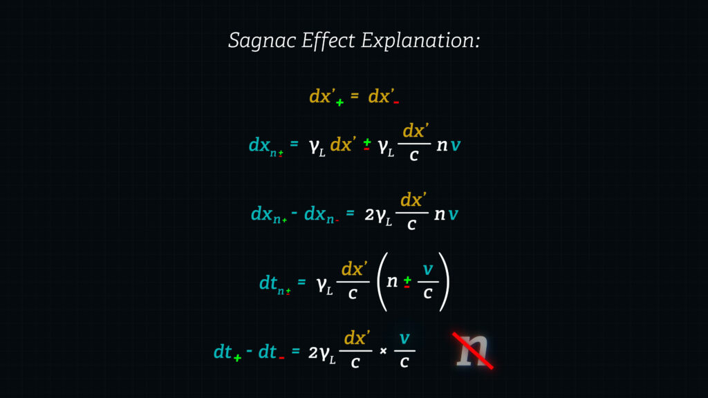
\(𝑑𝑡_+ − 𝑑𝑡_− (𝑆𝑎𝑔𝑛𝑎𝑐) = 𝛾𝐿 \frac{𝑑𝑥′}{𝑐} (𝑛 + \frac{𝑣}{𝑐}) − 𝛾𝐿 \frac{𝑑𝑥′}{𝑐} (𝑛 − \frac{𝑣}{𝑐}) = 2𝛾𝐿 \frac{𝑑𝑥′}{𝑐} ∗ \frac{𝑣}{𝑐} \)
Note that this produces a positive number. Meaning that it requires more time to travel a distance dx’ downstream than the time required to travel the same dx’ distance upstream.
Also note that there is no refractive index, n, in the final formula. The time difference for a Sagnac setup is not dependent on the refractive index of the medium.
Doesn’t this seem strange? If light is traveling at a slower speed through a refractive medium, why wouldn’t the difference in downstream versus upstream travel times be affected by the speed at which light is traveling?
Or in our river analogy, why wouldn’t the progress of the hovercraft downstream versus upstream be affected by the density of the obstructive logs floating in the river? We need to pick apart the formula for dt to better understand what’s going on.
Recall from Episode 9.5.A that it takes n times longer for light to travel a given distance, dx’, through a stationary refractive medium as compared to light traveling through vacuum.
\(𝑑𝑡′_{𝑣𝑎𝑐𝑢𝑢𝑚} = \frac{𝑑𝑥′}{𝑐} 𝑑𝑡′_{𝑟𝑒𝑓𝑟𝑎𝑐𝑡𝑖𝑜𝑛} = \frac{𝑛𝑑𝑥′}{𝑐} \)
Let’s use a mathematical trick and rewrite the refractive index as, n equals 1 plus n minus 1.
\(𝑛=1+(𝑛−1) \)
Now this formula might seem mathematically trivial, but its components have physical meaning.
\(𝑑𝑡′_{𝑟𝑒𝑓𝑟𝑎𝑐𝑡𝑖𝑜𝑛} = 1 ∗ \frac{𝑑𝑥′}{𝑐} + (𝑛−1) ∗ \frac{𝑑𝑥′}{𝑐} \)
According to our trivial equation, we have deconstructed the variable n, into a first term equal to 1 and a second term equal to (n-1).
1 times dx’/c is the time required for light to travel through a distance dx’ through vacuum. But when travelling through a refractive medium it takes more time. And so, we add that more time as the term (n-1) times dx’/c.
So, the incremental time required for light to travel through a refractive medium compared to time through vacuum is n minus 1, times dx’ over c.
\(𝑑𝑡′_{𝑟𝑒𝑓𝑟𝑎𝑐𝑡𝑖𝑜𝑛} = 𝑑𝑡′_{𝑣𝑎𝑐𝑢𝑢𝑚} + 𝑑𝑡′_{𝑖𝑛𝑐𝑟𝑒𝑚𝑒𝑛𝑡𝑎𝑙} \)
\(𝑑𝑡′_{𝑖𝑛𝑐𝑟𝑒𝑚𝑒𝑛𝑡𝑎𝑙} = 𝑑𝑡′_{𝑟𝑒𝑓𝑟𝑎𝑐𝑡𝑖𝑜𝑛}−𝑑𝑡′_{𝑣𝑎𝑐𝑢𝑢𝑚} \)
\(𝑑𝑡′_{𝑖𝑛𝑐𝑟𝑒𝑚𝑒𝑛𝑡𝑎𝑙} = [ 1 ∗ \frac{𝑑𝑥′}{𝑐} + (𝑛−1) ∗ \frac{𝑑𝑥′}{𝑐}] − 1 ∗ \frac{𝑑𝑥′}{𝑐} \)
\(𝑑𝑡′_{𝑖𝑛𝑐𝑟𝑒𝑚𝑒𝑛𝑡𝑎𝑙} = 1 ∗ \frac{𝑑𝑥′}{𝑐} + 𝑛 \frac{𝑑𝑥′}{𝑐} − \frac{𝑑𝑥′}{𝑐} − 1 ∗ \frac{𝑑𝑥′}{𝑐} \)
\(𝑑𝑡′_{𝑖𝑛𝑐𝑟𝑒𝑚𝑒𝑛𝑡𝑎𝑙} = 𝑛 \frac{𝑑𝑥′}{𝑐} − \frac{𝑑𝑥′}{𝑐} \)
\(𝑑𝑡′_{𝑖𝑛𝑐𝑟𝑒𝑚𝑒𝑛𝑡𝑎𝑙} = (𝑛−1) \frac{𝑑𝑥′}{𝑐} \)
Now let’s take our formula for time elapsed when light passes through a refractive medium in the stationary frame,
\(𝑑𝑡_{𝑛±} = 𝛾𝐿 \frac{𝑑𝑥′}{𝑐} (𝑛± \frac{𝑣}{𝑐}) \)
and separate n into its vacuum term, 1, and its incremental term, n minus 1.
\(𝑑𝑡_{𝑛±} = 𝛾𝐿 \frac{𝑑𝑥′}{𝑐} ( 1 + (𝑛−1) ± \frac{𝑣}{𝑐}) \)
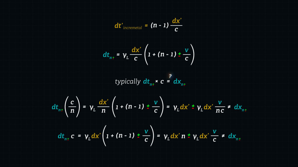
Now, typically, when we multiply elapsed time in the stationary frame, dt, by speed in the stationary frame, c, we obtain distance traveled in the stationary frame, dx.
𝑡𝑦𝑝𝑖𝑐𝑎𝑙𝑙𝑦 \(𝑑𝑡_{𝑛±} ∗ 𝑐 = 𝒅𝒙_{𝒏±} \)
But if we were to multiply our formula for time elapsed times light speed c, we will not obtain Lorentz’s formula for dx.
\(𝑑𝑡_{𝑛±} 𝑐 = 𝛾𝐿 𝑑𝑥′ (1+(𝑛−1) ± \frac{𝑣}{𝑐}) = 𝛾𝐿 𝑑𝑥′ 𝑛± 𝛾𝐿 𝑑𝑥′ \frac{𝑣}{𝑐} ≠ 𝑑𝑥_{𝑛±} \)
In other words, something is deviating from Special Relativity. Why? Because the speed of light through a refractive medium is not a constant speed c.
What if we were to multiply our formula times c divided by n, shouldn’t that produce the Lorentz formula for distance dx?
\(𝑑𝑡_{𝑛±} (\frac{𝑐}{𝑛}) = 𝛾𝐿 \frac{𝑑𝑥′}{𝑛} (1+(𝑛−1) ± \frac{𝑣}{𝑐}) = 𝛾𝐿 𝑑𝑥′±𝛾𝐿𝑑𝑥′ \frac{𝑣}{𝑛𝑐} ≠ 𝑑𝑥_{𝑛±} \)
The answer again is no.
This means that the stationary-Frame Speed of light traveling through a moving refractive medium is neither speed c nor speed c divided by n.
Think about that. It seems a bit contradictory, right?
But what if we do the following?
Let’s break down the time formula into three terms.
\(𝑑𝑡_{𝑛±} = 𝛾𝐿 \frac{𝑑𝑥′}{𝑐} (1+(𝑛−1)± \frac{𝑣}{𝑐}) \)
Let’s look at the first term γL (gamma_L) times dx’ over c.
\(𝑑𝑡_{𝑛±} = 𝛾𝐿 \frac{𝑑𝑥′}{𝑐} + 𝛾𝐿 \frac{𝑑𝑥′}{𝑐} (𝑛−1) ± 𝛾𝐿 \frac{𝑑𝑥′}{𝑐} \frac{𝑣}{𝑐} \)
To this term, we attribute the stationary frame time required for light to travel distance dx’ through vacuum. If we multiply it by light speed, c, we get the average distance traveled when measured with stationary frame markers.
\(𝑑𝑥_{𝑡𝑒𝑟𝑚 1} = 𝛾𝐿 \frac{𝑑𝑥′}{𝑐} ∗ 𝑐 = 𝑑𝑥_{𝑎𝑣𝑒𝑟𝑎𝑔𝑒} = \frac{𝑑𝑥_+ + 𝑑𝑥_−}{2} \)
In our river analogy, this would be the average of the stationary frame distances the two hovercraft would travel if they both had begun their trips starting at a single moving clock, and traveled around the lazy river a distance dx’ in the absence of logs until each hovercraft returned to that same moving clock.
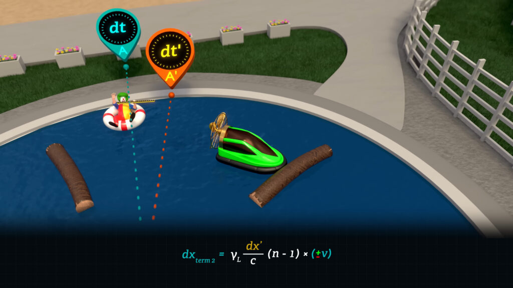
Next, we take and isolate the second term of our time formula,
\(𝑑𝑡_{𝑛±} = 𝛾𝐿 \frac{𝑑𝑥′}{𝑐} + 𝛾𝐿 \frac{𝑑𝑥′}{𝑐} (𝑛−1) ± 𝛾𝐿 \frac{𝑑𝑥′}{𝑐} \frac{𝑣}{𝑐} \)
which we have associated with light being blocked by refractive molecules, and multiply it by the speed of those molecules v, to solve for that component of stationary frame distance traveled.
\(𝑑𝑥_{𝑡𝑒𝑟𝑚 2} = 𝛾𝐿 \frac{𝑑𝑥′}{𝑐} ∗ (𝑛−1)∗(±𝑣) \)
In other words, if we assume that a light signal is somehow delayed by or absorbed by the refractive molecules for an amount of time that is proportional to n minus 1, then it will travel a certain distance during that amount of time.
We know that the refractive molecules (or the logs on the river) are moving at speed v with respect to the stationary frame. So, during the time that the light signal is delayed by these molecules, the light signal travels at speed v, not speed c or speed c divided n.
In our hovercraft analogy, this would be the speed of the hovercraft with respect to the land when the hovercraft is being impeded by a log in the river.
Finally, we take the third term of our time formula,
\(𝑑𝑡_{𝑛±} = 𝛾𝐿 \frac{𝑑𝑥′}{𝑐} + 𝛾𝐿 \frac{𝑑𝑥′}{𝑐} (𝑛−1) ± 𝛾𝐿 \frac{𝑑𝑥′}{𝑐} \frac{𝑣}{𝑐} \)
which we associate with the longer distance that our light signal must travel to “catch” a moving distance marker when the signal travels downstream, or the shorter distance that our light signal will travel to “collide” with an oncoming moving distance marker as the light signal moves upstream.
We multiply this third term times lightspeed c because our light signal is moving this differential distance in between obstructing refractive molecules; so, it is moving between molecules at its normal speed 𝑐.
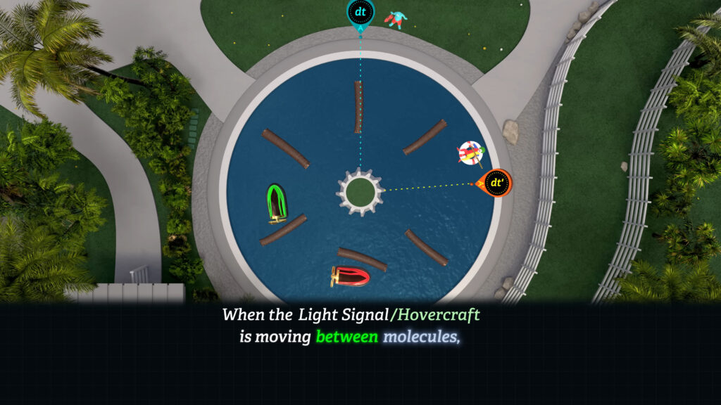
\(𝑑𝑥_{𝑡𝑒𝑟𝑚 3} = ± 𝛾𝐿 \frac{𝑑𝑥′}{𝑐} ∗ \frac{𝑣}{𝑐} ∗ 𝑐 \)
Now if we add these three terms together, what do we get?
By having multiplied the second time-term by v instead of by c, or instead of by c over n, we see that two of the expanded terms will cancel, leaving the dx’ term plus or minus a term that is a function of refractive index n times v.
\(𝑑𝑥_± = 𝛾𝐿 \frac{𝑑𝑥′}{𝑐} ∗ 𝑐 + 𝛾𝐿 \frac{𝑑𝑥′}{𝑐} ∗ (𝑛−1) ∗ (±𝑣) ± 𝛾𝐿 \frac{𝑑𝑥′}{𝑐} ∗ \frac{𝑣}{𝑐} ∗ 𝑐 \)
\(𝑑𝑥_± = 𝛾𝐿 𝑑𝑥′± 𝛾𝐿 \frac{𝑑𝑥′𝑛}{𝑐} 𝑣 ∓ 𝛾𝐿 \frac{𝑑𝑥′}{𝑐} 𝑣± 𝛾𝐿 \frac{𝑑𝑥′}{𝑐}𝑣 \)
\(𝑑𝑥_± = 𝛾𝐿 𝑑𝑥′ ± 𝛾𝐿 \frac{𝑑𝑥′𝑛}{𝑐}𝑣 \)
And since dx’ times n over c is equal to dt’,
\(\frac{𝑑𝑥′𝑛}{𝑐} = 𝑑𝑡′ \)
this reduces to the Lorentz transform for dx.
\(𝛾𝐿(𝑑𝑥′±𝑣∗𝑑𝑡′)= 𝑑𝑥_± \)
In other words, by multiplying the first and third terms of the time formula by c, and the second term by v, we obtain Lorentz’s stationary frame distance traveled by light.
And the difference in the distance dx traveled in the downstream versus upstream directions will be, two times the Lorentz gamma factor times dx’ divided by c times n times v.
\(𝑑𝑥_{𝑛+} − 𝑑𝑥_{𝑛−} = 2𝛾𝐿 \frac{𝑑𝑥′}{𝑐} 𝑛𝑣 \)
All of this should cause you to think for a minute.
This analysis suggests that when the light signal (or hovercraft) is moving between molecules, it moves at speed c, or speed c-sub-h for hovercraft. But when the light signal (or hovercraft) is hindered by molecules (or logs) it moves at speed v, not at speed c, nor at speed c-sub-h, nor at speed c divided by n.
This suggests that light is being temporarily obstructed by refractive molecules for a fraction of the time. And this fraction is proportional to the refractive index minus 1. Otherwise, light moves between the molecules of the refractive medium at its normal speed c.
Grant Sanderson has presented a model based on Richard Feynman’s lectures suggesting that wave interference accounts for the slowing of light speed in refractive media. This model proposes a phase shift created by some type of “kick” due to the oscillation of electrons in the refractive media.
But the model, as presented, looks only at stationary refractive media. If such a model were to be extended to moving refractive media, it will not only have to explain how that “kick” decreases light speed in one direction, but that same “kick” must increase light speed in the opposite direction. And why that difference in light speed does not result in a simple linear addition of the speed of the medium; but rather a more complex blend of an incremental speed-v effect coupled with a differential v-over-c effect.
Moreover, such a wave model will need to explain why such incremental “kicks” have no effect on the outcome of a Sagnac experiment.
A similar model for light traveling through a stationary refractive medium has been developed by Jorge Diaz using a quantum mechanical approach. If extended to moving refractive media, it also must explain non-linear, differential light speed in both the stationary and moving frames, and why a Sagnac result is not impacted by the presence of the proposed wave interference.
I’m not saying it can’t be done, but it’s an interesting challenge to anyone who tackles it.
Now that we’ve analyzed the travel times, lets switch gears and look at overall light speeds. We can take our formula for dx sub-n-plus or minus and divide by our formula for dt sub-n plus or minus.
\(\frac{𝑑𝑥_{𝑛±}}{𝑑𝑡_{𝑛±}} = \frac{𝛾𝐿 (𝑑𝑥′±𝑣𝑑𝑡′)}{𝛾𝐿(\frac{𝑑𝑥′𝑛}{𝑐} ± \frac{𝑣𝑑𝑥′}{𝑐^2})} \)
If we divide top and bottom by dt’ and cancel terms we get the following.
\(\frac{𝑑𝑥_{𝑛±}}{𝑑𝑡_{𝑛±}} = \frac{\frac{𝑐}{𝑛} ± 𝑣}{1 ± \frac{𝑣}{𝑐𝑛}} \)
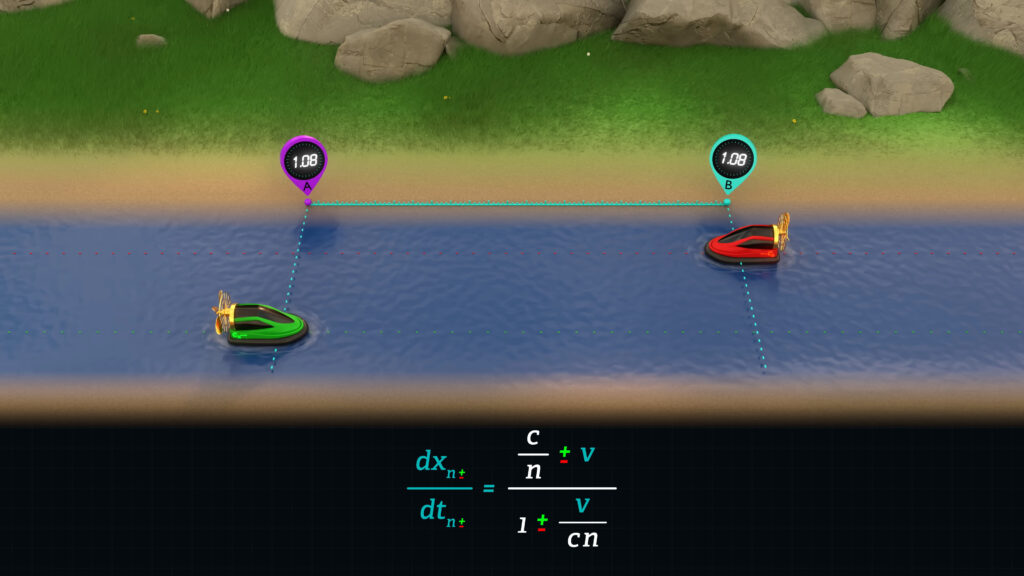
For those of you who watched Episode 9.3 you might recognize this as von Laue’s relativistic velocity addition formula for light traveling through refractive media in the stationary frame. This formula is valid for computing times in the stationary frame, because clocks in the stationary frame report the same time of day when synchronized using Einstein’s clock synchronization method.
And so, von Laue’s formula, and the underlying stationary frame Lorentz transform work in this frame.
But the same is not true in the moving frame, where Einstein’s method produces clocks that report different times of day.
The failure of the Lorentz transforms is revealed when we provide only one clock to make all clock measurements. A single clock cannot be manipulated by Einstein’s method of clock offset, and so von Laue’s formula and the Lorentz transforms fail in the moving frame when only one clock is used.
Now, as we covered in Episode 9.5.A, if our setup has only one clock, we must use the Tangherlini dt’-transforms to compute times, distances, and speeds in the moving frame rather than the Lorentz transforms.
To compute the speed of light in the moving frame, we recall that distance dx’ is constant in a Sagnac setup, because the beam splitter circulates with the moving frame, and so dx’ / dt’ sub-star-n plus or minus is equal to dx’ divided by the Tangherlini formula for dt’,
\(\frac{𝑑𝑥′}{𝑑𝑡′_{∗𝑛±}} = \frac{𝑑𝑥′}{\frac{𝑑𝑡_{𝑛±}}{𝛾𝐿}} \)
\(𝑑𝑡_{𝑛±} = 𝛾𝐿 \frac{𝑑𝑥′}{𝑐′_{𝑡𝑤𝑎}} (𝑛± \frac{𝑣}{𝑐}) \)
which is our stationary frame formula for dt sub n plus or minus over gamma.
\(𝑑𝑡_{𝑛±} / 𝛾𝐿 = \frac{𝑑𝑥′}{𝑐′_{𝑡𝑤𝑎}} (𝑛± \frac{𝑣}{𝑐}) \)
\(\frac{𝑑𝑥′}{𝑑𝑡′-{𝑛±}} = \frac{𝑑𝑥′}{\frac{𝑑𝑥′}{𝑐′_{𝑡𝑤𝑎}} (𝑛± \frac{𝑣}{𝑐})} \)
Which then simplifies to, the time-weighted average of light speed in vacuum divided by the refractive index, n, plus or minus v divided by c.
\(\frac{𝑑𝑥′}{𝑑𝑡′_{𝑛±}} = \frac{𝑐′_{𝑡𝑤𝑎}}{𝑛±\frac{𝑣}{𝑐}} = 𝑐′_{∗𝑛±} \)
As we showed in Episode 9.5.A the time weighted average of light speed in any moving reference frame is numerically equivalent to speed c, and so the formula for direction-dependent light speed in the moving reference frame is c divided by n plus or minus v divided by c.
\(𝑐′_{∗𝑛±} = \frac{𝑐}{𝑛 ± \frac{𝑣}{𝑐}} \)
This shows that light speeds are different in the plus and minus directions relative to the moving frame, depending on the speed v of the moving frame.
This is not what von Laue nor Einstein concluded because their models used either two-way light speeds (which we showed in Episode 9.5.A always produced a time-weighted average light speed of c divided by n); or they used two or more rigged clocks that distorted the measurement of one-way elapsed time.
In other words, as we covered in Episode 9.5.A, one-way light speed is not constant in the moving frame, regardless of the index of refraction; and this non-isotropy is absolutely necessary to obtain a fringe shift in a Sagnac setup.
Sorry, I don’t want to be sarcastic, but I simply cannot understand how physicists can look at the Sagnac result, particularly the linear Sagnac result that I refered to in episode 9.5.A, and not understand that light travels at different speeds in both the stationary and moving reference frames. This must be true, since the shifting of the interference pattern is a frame-independent observation.
The two counter propagating light signals must travel at different speeds in both the stationary and moving reference frames in order for there to be an interference pattern fringe shift.
So, before we move on to the Fizeau experiment, let’s summarize.
In a Sagnac setup, the distance, dx’, that light signals travel in the moving frame is the same in both directions;
\(𝑑𝑥′_+ = 𝑑𝑥′_− \)
whereas the distance, dx,
\(𝑑𝑥_{𝑛±} = 𝛾𝐿 𝑑𝑥′ ± 𝛾𝐿 \frac{𝑑𝑥′}{𝑐} ∗𝑛∗𝑣 \)
that the light signals travel in the stationary frame is variable, and depends on the refractive index and the speed v of the moving frame.
And the difference in the downstream versus upstream distances traveled in the stationary frame is a function of distance dx’, refractive index n, and the speed of the moving frame v.
\(𝑑𝑥_{𝑛+} − 𝑑𝑥_{𝑛−} = 2𝛾𝐿 \frac{𝑑𝑥′}{𝑐} ∗𝑛∗𝑣 \)
In contrast, the stationary frame time for the signal to travel a distance dx’ is a function of the distance dx’, the refractive index n, and the speed of the moving frame v.
However, the difference in the stationary frame time required for the downstream versus upstream signals to travel a distance dx’ will be a function of dx’ and v, but not the refractive index n.
𝑆𝑎𝑔𝑛𝑎𝑐: \(𝑑𝑡_+ − 𝑑𝑡_− = 2𝛾𝐿 \frac{𝑑𝑥′}{𝑐}∗ \frac{𝑣}{𝑐} \)
So, why might this be so? Well, when a light signal travels a fixed distance dx’ in the moving frame, the downstream signal will encounter the same number of refractive molecules (or logs in our river analogy) as the upstream signal. And thus, the difference in time elapsed will be independent of the density of the refractive molecules.
The hovercraft traveling a moving frame distance dx’ upstream will encounter the same number of logs as the hovercraft traveling the same moving frame distance dx’ downstream. And so, a Sagnac fringe shift will be the same for vacuum as it is for any refractive medium.
In our lazy river analogy, Fizeau would have both hovercraft travel in opposite directions from the stationary marker on the bank of the river around to the same marker.
Both hovercraft travel the same stationary frame distance dx.
So, let’s write the formula for elapsed time in the upstream and downstream directions as a function of dx.
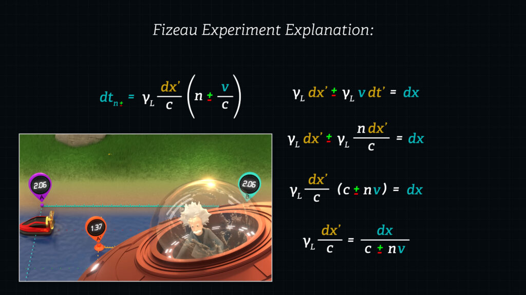
We can first take our time formula,
\(𝑑𝑡_{𝑛±} = 𝛾𝐿 \frac{𝑑𝑥′}{𝑐} (𝑛 ± \frac{𝑣}{𝑐}) \)
and then rewrite it in terms of dx by using Lorentz’s stationary frame distance transform to solve for gamma times dx’ divided by c.
\(𝛾𝐿 𝑑𝑥′±𝛾𝐿𝑣𝑑𝑡′=𝒅𝒙 \)
\(𝛾𝐿𝑑𝑥′±𝛾𝐿𝑣 \frac{𝑛𝑑𝑥′}{𝑐} =𝑑𝑥 \)
\(𝛾𝐿 \frac{𝑑𝑥′}{𝑐} (𝑐±𝑛𝑣)=𝑑𝑥 \)
\(𝛾𝐿 \frac{𝑑𝑥′}{𝑐} = \frac{𝑑𝑥}{𝑐± 𝑛𝑣} \)
The Lorentz transform for distance in the stationary frame is valid here since clocks report the same time of day in the stationary frame. It is only in the moving frame that we need to be cognizant of clock offsets.
We see that we can replace the Lorentz gamma factor times dx’ over c with dx over c plus or minus n time v.
\(𝑑𝑡_{𝑛±} = \frac{𝑑𝑥}{𝑐±𝑛𝑣}(𝑛±\frac{𝑣}{𝑐}) \)
If we subtract the upstream elapsed time from the downstream elapsed time, we get, negative 2 times v times dx times the ratio of 1 minus one over n squared all over c squared over n squared minus v squared.
𝐹𝑖𝑧𝑒𝑎𝑢: \(𝑑𝑡_{𝑛+} − 𝑑𝑡_{𝑛−} = −2𝑣𝑑𝑥 \frac{1−\frac{1}{𝑛^2}}{\frac{𝑐^2}{𝑛^2}−𝑣^2} \)
It’s much more complicated than the Sagnac result.
𝑆𝑎𝑔𝑛𝑎𝑐: \(𝑑𝑡_+ − 𝑑𝑡_− = 2𝛾𝐿 \frac{𝑑𝑥′}{𝑐} ∗ \frac{𝑣}{𝑐} \)
We see that the difference in elapsed time for the downstream versus upstream signals is a function of the refractive index, n, and this is what is found in a Fizeau experiment.

Also note that it will take more time to travel the distance dx upstream than downstream. In other words, the green hovercraft travels downstream faster than the red hovercraft travels upstream in a Fizeau setup. That’s opposite of what we found in a Sagnac setup.
We can perform the same analysis for the Fizeau effect as we did for the Sagnac effect where we deconstructed the refractive index into two components.
\(𝑑𝑡_{𝑛±} = \frac{𝑑𝑥}{𝑐±𝑛𝑣}(1+(𝑛−1)± \frac{𝑣}{𝑐}) \)
\(𝑑𝑡_{𝑛±} = \frac{𝑑𝑥}{𝑐±𝑛𝑣} + \frac{𝑑𝑥}{𝑐±𝑛𝑣} (𝑛−1) ± \frac{𝑑𝑥}{𝑐±𝑛𝑣} \frac{𝑣}{𝑐} \)
And so, we can treat the three terms of the time formula as we did in the Sagnac analysis, where we multiply the first term by speed c,
\(\frac{𝑑𝑥}{𝑐±𝑛𝑣} ∗ 𝑐 \)
the second term times the speed of the refractive molecules, plus or minus v,
\(\frac{𝑑𝑥}{𝑐±𝑛𝑣} ∗ (𝑛−1)∗(±𝑣) \)
and the third term times speed c.
\(± \frac{𝑑𝑥}{𝑐±𝑛𝑣} ∗ \frac{𝑣}{𝑐} ∗ 𝑐 \)
When we combine these three terms we simply get the distance dx.
\(𝑑𝑥(\frac{𝑐}{𝑐±𝑛𝑣}± \frac{𝑛𝑣}{𝑐±𝑛𝑣})=𝑑𝑥 \)
In other words, when we multiply the three terms of the Fizeau time formula by the appropriate speeds of the light signal corresponding to each term, we get the stationary frame distance, dx. Which is what we would expect when we multiple time by speed.
And so, even though the Fizeau setup controls laboratory frame path length, and the Sagnac setup controls moving frame path length, they both operate by the same molecular principles where light can be treated as traveling at speed c between molecules and at speed v when obstructed by molecules.
With this model we can perfectly predict elapsed times and travel distances for both the Fizeau and Sagnac setups.
It’s important to appreciate that the Fizeau result is affected by refractive index, because the light signal encounters more refractive molecules when traveling upstream a fixed distance dx in a laboratory frame, and fewer refractive molecules when traveling downstream a fixed distance dx in a laboratory frame.
Whereas a light signal in a Sagnac experiment encounters the same number of refractive molecules when traveling the same moving frame distance, dx’, in either direction.
OK, before I wrap this up, I’d like to ask you not to get hung up on whether light behaves light a particle or like a wave. That’d be like arguing over whether Ironman or Batman is the stronger superhero. The particle/wave debate has gone on for decades if not centuries, and even though there are staunch supporters for each model, neither model explains everything perfectly. The conclusions reached in this episode transcend that debate.

What I’ve demonstrated here, perhaps for the first time ever, is that refractive barriers encountered along the light path, whether you want to envision those barriers to be molecules or fields created by the oscillations of charged particles, impart their speed to the light signal for a fraction of the total elapsed time, and such fraction is proportional to the refractive index.
I’ve also shown that the light signal pauses during those encounters, and during those pauses the light signal moves at the speed at which those barriers are moving relative to the stationary frame, not at speed c. That’s the take-home message.
Lastly, I’d like to explain why I developed this episode using Special Relativity, even though most of you know I believe that Special Relativity is flawed. Well, just as in Episode 9.8 where I used the equations of Special Relativity to reveal that both Galilean and Einsteinian relativity are both flawed concepts.
I again use Einstein’s own tools here to show that light travels at different speeds relative to the moving reference frame. This directly challenges the fundamental postulates of Special Relativity.
I could have taken a non-relativistic approach, or used my own hybrid relativistic model to arrive at essentially the same fringe shifts.
But I’ve found that in order to seize the attention of the masses of devoted Einsteinians, I need to adhere strictly to the rules of Special Relativity. I mean, one must travel through the Land of Oz to expose the man behind the curtain, right?
OK, that’s it for now. If you have any questions, please write them in the comments section. And if I’ve caused you to think outside the box, please rate this video favorably. I’m Joe Sorge, and thanks for watching.