Welcome to Ask Us Whatever. I’m your host, Joe Sorge
Before we begin, a word of caution. I’m going to deviate from orthodox teachings in this episode. The questions I’m about to raise and the answers I’m about to raise and the answers I’m going to provide are going to seem radical. Most people think that special relativity has been proved beyond a shadow of a doubt. Experimental results have been remarkably consistent with the theory. And, as far as I know, no one has proposed a better theory – at least until now. I know, that’s a bold claim. But if you think I’ve done a decent job in this series so far, give me a chance. I promise, the upcoming model is going to be logically consistent, significantly more plausible than special relativity, and will conform to experimental results as well or better than special relativity. And for those of you who have an inquisitive mind and appreciate creative solutions to difficult problems, the challenge I’m about to throw down to special relativity is going to be exciting.
Alright, to briefly recap, Lorentz derived equations to compute the distance that objects travel from the perspective of both stationary and moving observers, and he used these equations, called “distance and time transformations”, to explain the Michelson Morley result. Einstein arrived at essentially the same transformations and incorporated them into his special theory of relativity. We’re going to re-derive analogs to these equations, but without using length contraction, as an alternative way to explain the Michelson Morley result.
There are many reasons why length contraction is not an attractive solution. First of all, in order to be compatible with the Michelson Morley result, and with special relativity theory, length contraction needs to be real, a real physical event. It cannot be merely a virtual concept or illusion. Lengths do have to contract under the theory. And if length contraction really happens, we all need to shrink, in real time, along the axis of the Earth’s motion, but not in the other two dimensions.

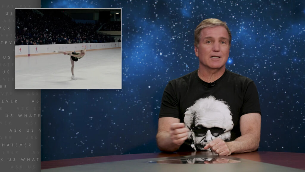
Every time we twist or turn, our bodies need to contract in one dimension and expand in the other. A figure skater performing an axel-move must rapidly undergo contraction and expansion. An airplane propeller moving diagonally with respect to the Earth’s motion must contract and re-expand with every partial turn of its blades. Materials such as steel must contract just as quickly and easily as marshmallows and do so without requiring extra energy.
When Lorentz incorporated the concept of length contraction into his distance and time transformations, it provided an elegant mathematical symmetry to some very complicated concepts. The mathematics were seductive, and that has probably helped length-contraction survive as long as it has. But I’m going to show that there are significant inconsistencies when these transformations are applied to the Doppler effect, light aberration, and the Fizeau experiment; and that experimental results produced to date have either not been sensitive enough to reveal the problems, or have been explained away using circular logic.
I call my alternative – the Alternative Model.

And I want to apologize up front; we’re going to need to do a little bit of math to lay out the model. You know, the skeptics are never going to be convinced otherwise, but I’ll try to do it in a way that doesn’t put us all to sleep.
Alright, let’s start from scratch. We’ll ignore for the moment Einstein’s postulates, and we’ll also dispense with length contraction. But since we showed in Episode 3 that the slowing of light clocks makes sense, let’s hold on to that concept.

Recall that light clocks in the moving frame of reference tick slower than stationary clocks. In order to keep track of time and distance in the stationary and moving frames, we are going to use a shorthand similar to what is used in calculus (but not as difficult).
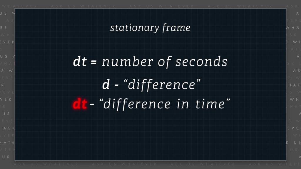
\(dt = \text{number of seconds} \)
\(dt \) will represent the number of stationary frame seconds that elapse on a stationary clock between the start and end of an event
The letter “d” just stands for “difference”. \(dt \) is a “difference in time” as measured in seconds.
\(dt’ \) will represent the number of moving frame seconds\(’ \) that elapse on a clock within the moving frame
\(dt’ = \text{number of seconds}’ \)
Einstein assumed that moving frame clocks tick
\(dt’ = \frac{dt}{\gamma} \)
slower than stationary clocks by the Lorentz \(\gamma \) factor. So if the same event is measured with a stationary clock and a moving clock, the moving clock will record \(\gamma \)-fold fewer

Now, since we are relaxing some of the constraints of special relativity, the possibility exists that time does not dilate according to the Lorentz \(\gamma \) factor. It might, but it might not. So, for now, let’s replace the Lorentz time dilation \(\gamma \) factor with the Greek letter \(\tau \),
\(dt’ = \frac{dt}{\tau} \)
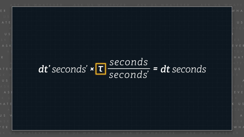
\(dt’ \space \text{seconds}’ \times \tau \frac{seconds}{second’} = \)
\(dt \space \text{seconds} \)
So, \(dt’ \) seconds\(’ \) times \(\tau \) seconds per second\(’ \) equals \(dt \) seconds. If it turns out that \(\tau \) is the same as the Lorentz \(\gamma \) factor, we’ve done no harm.
Let’s also break with orthodox doctrine and allow light to possibly travel at speeds other than \(c \). I know this sounds ludicrous, but bear with me – you’ll see that it all comes together as we get into this.
We will assign a variable function, \(\gamma_\phi \), to light speed,
\(\gamma_{\phi}c \)
So, light speed can be \(\gamma_\phi \) times \(c \). If it turns out that \(\gamma_\phi \) is just the number 1, then light speed will be the constant \(c \), and we’ve done no harm. But if light speed is not constant, we have \(\gamma_\phi \) to keep track of it.
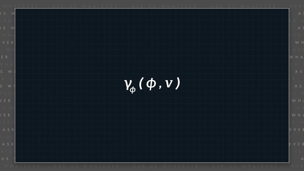
\(\gamma_\phi \) can be a function of both the angle, \(\phi \), at which light is emitted relative to the axis of motion, and the speed of the inertial reference frame, \(v \).
\(\gamma_{\phi}(\phi, v) \)
The speed of light in the longitudinal, or \(x \)-direction, which we will call \(c_x \), would be \(\gamma_\phi \) at a zero degree angle, times \(c \).
\(c_x = \gamma_{\phi}(0^{\circ}, v)\times c \)
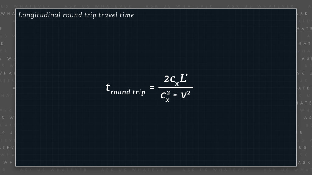
Let’s rewrite the textbook formula to compute round trip longitudinal travel time. We will use \(c_x \) instead of \(c \) to remind us that the speed of light in the \(x \)-direction might not be \(c \).
\(t_{round \space trip} = \frac{L’}{c_{x}-v}+\frac{L’}{c_{x}+v} = 2\frac{c_xL’}{c^2_x-v^2} \)
Longitudinal travel time equals \(L’ \), the proper length of the train car, divided by \(c_x \) minus \(v \) plus \(L’ \) divided by \(c_x \) plus \(v \). And if we combine the fractions, we obtain 2 times \(c_x \) times \(L’ \) all divided by \(c_x \) squared minus \(v \)-squared. If this formula seems foreign, please watch Episode 2 on clock synchronization for a review.
If it turns out that light simply travels at speed \(c \) in the \(x \)-direction, then our equation will simply revert to the textbook formula for round-trip travel time.
Now, let’s divide numerator and denominator by \(c^2_x \). Here’s some fast algebra and you can pause the video to examine it carefully.
\(t_{round \space trip} = 2\frac{L’}{c_x} \times \frac{1}{(1-\frac{v^2}{c^2_x})} \)
We get 2 times \(L’ \) divided by \(c_x \) times the quantity 1 divided by 1 minus \(v \) squared over \(c_x \) squared. The fraction on the right is the Lorentz \(\gamma \) factor squared, but with light speed of \(c_x \) in place of \(c \). We will call this variant of the Lorentz factor \(\gamma_s \), instead of \(\gamma \),
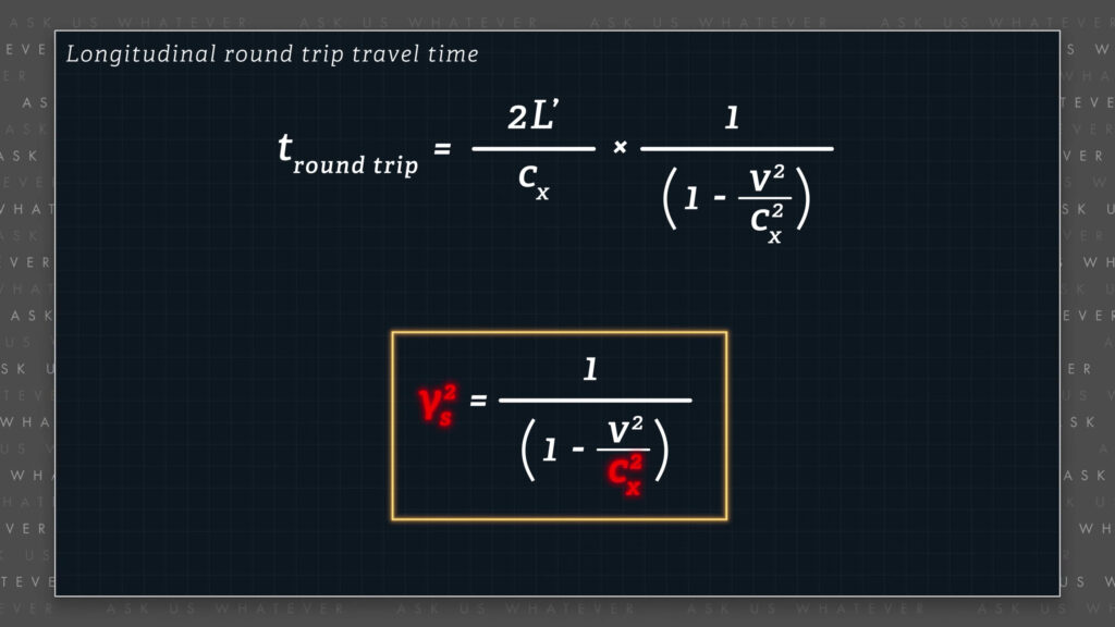
\(\gamma_s = \frac{1}{\sqrt{1-\frac{v^2}{c^2_x}}} \)
Again, if \(c_x \) turns out to be just the constant \(c \), then \(\gamma_s \) will simply be the Lorentz \(\gamma \) factor; and our formula for round trip longitudinal travel time will agree with the textbook formula. No harm done.
Okay, so using our new notation,
\(t_{round \space trip, \space longitudinal} = 2\frac{L’}{c_x}\gamma^2_s \)
the round trip, longitudinal travel time equals 2 times \(L’ \) divided by \(c_x \) times \(\gamma_s \) squared.
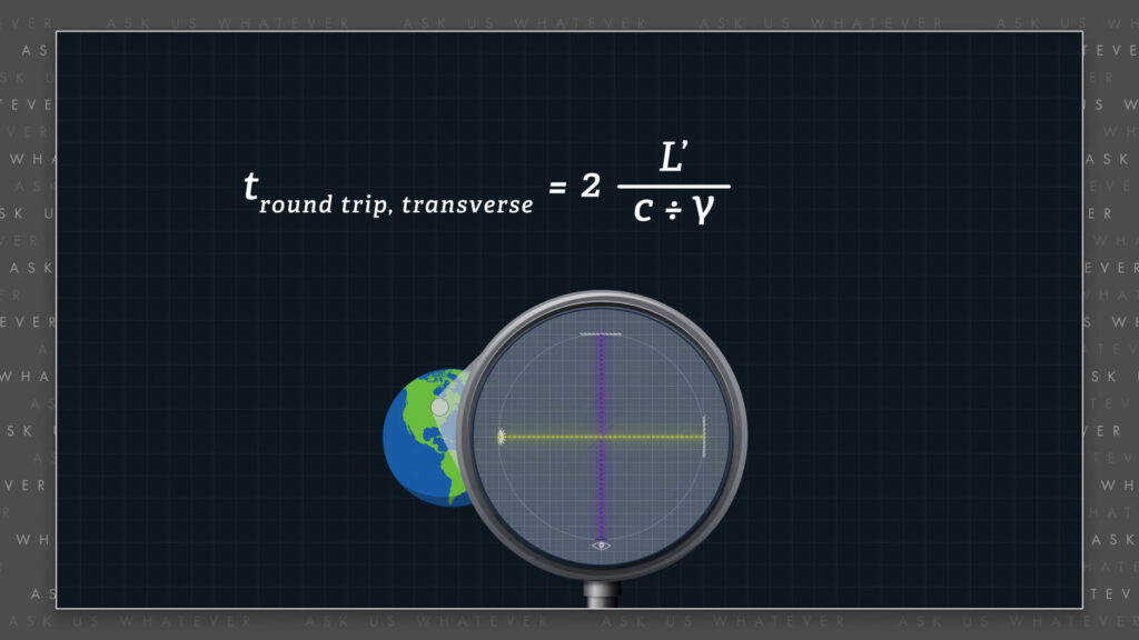
Now, Lorentz and Einstein believed that the round trip time required for light to travel a path transverse to the direction of Earth’s motion was
\(t_{round \space trip, \space transverse, \space Einstein} = 2\frac{L’}{\frac{c}{\gamma}} = \)
\(2\frac{L’\gamma}{c} \)
two times the transverse path length, which we will call \(L’ \) since Michelson and Morley used equal-length transverse and longitudinal light paths, divided by the transverse component of light speed, which Einstein believed is \(c \) divided by \(\gamma \).
This can be re-written as 2 times \(L’ \) times \(\gamma \) divided by \(c \).
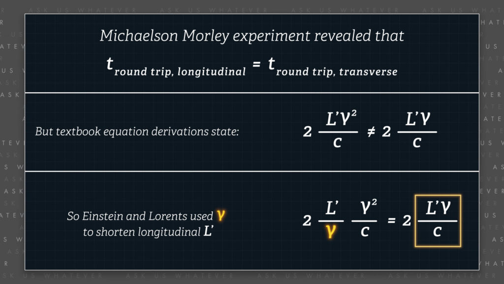
Recall that the Michelson Morley experiment unexpectedly revealed that the round trip time required for light to travel the longitudinal path was equal to the round trip time for light to travel the transverse path. And this created a dilemma because if light traveled at a constant speed \(c \), then something was wrong with the textbook equations for the longitudinal and transverse travel times,
\(2\frac{L’\gamma^2}{c} \neq 2\frac{L’\gamma}{c} \)
\(\text{(Textbook travel times} \)
\(\text{are not equal.)} \)
since those formulas do not produce identical answers.
You might recall that Lorentz and Einstein conjured up the concept of length contraction to transform this inequality into an equality by proposing that \(L’ \) contracts by one factor of \(\gamma \) in the direction of motion. They essentially plugged in what some might call a fudge factor of \(\gamma \) into the denominator so that
\(2\frac{L’}{\gamma}\frac{\gamma^2}{c} = 2\frac{L’\gamma}{c} \)
two times the contracted distance, \(L’ \) over \(\gamma \), times \(\gamma \) squared over \(c \), would equal 2 times \(L’ \) times \(\gamma \) over c: the time predicted by the Michelson Morley experiment.
But what if length contraction is not the answer? As we’ve discussed, it’s a very, very implausible explanation. So let’s see what happens if we equate our formulas for round trip longitudinal and transverse travel times.
\(t_{round \space trip} = \frac{2L’\gamma^2_s}{c_x} = \frac{2L’}{\frac{c}{\tau}} \)
We set two times \(L’ \) times \(\gamma^2_s \) divided by the \(x \)-component of light speed \(c_x \), equal to two times \(L’ \) divided by our transverse component of light speed: \(c \) divided by our time-dilation factor \(\tau \).
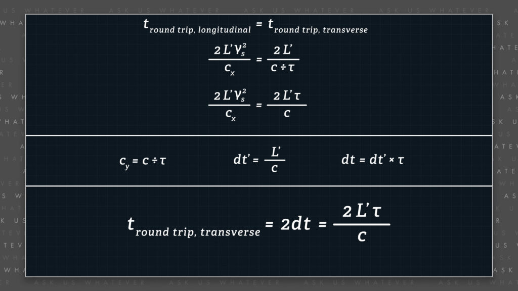
\(t_{round \space trip} = \frac{2L’\gamma^2_s}{c_x}=\frac{2L’\tau}{c} \)
The latter formula can be rearranged to be 2 times \(L’ \) times \(\tau \) divided by \(c \).
Note that the transverse component of light speed, which we also have called \(c_y \) in prior episodes, must, by definition, be \(c \) divided by \(\tau \). This is because \(dt’ \) in the moving frame is equal to
\(dt’ = \frac{L’}{c} \)
the transverse distance, \(L’ \), divided by \(c \). And by definition, \(dt \) is equal to \(dt’ \) times \(\tau \)
\(dt = dt’\tau \)
and therefore round trip transverse travel time must be equal to two times \(L’ \) times \(\tau \) divided by \(c \).
\(t_{round \space trip} = 2dt = 2\frac{L’\tau}{c} \)
Now if we cancel the 2 times \(L’ \) terms from both sides of our equation for round trip travel time,
\(t_{round \space trip} = 2\frac{L’\gamma^2_s}{c_x} = 2\frac{L’\tau}{c} \)
\(\frac{\gamma^2_s}{c_x} = \frac{\tau}{c} \)
we end up with one equation and two unknowns, \(\gamma_s \) squared divided by \(c_x \) equals \(\tau \) divided by \(c \); the two unknowns are \(c_x \) and \(\tau \) (remember that \(\gamma_s \) is a function of speed \(v \), which we know, and \(c_x \); so \(\gamma_s \) will not be an unknown once we know \(c_x \)).
Since we do not yet know much about \(\tau \) and \(c_x \), we have to make an assumption at this point. The assumption may turn out to be correct, or it may be wrong. Experimental results will determine that. But for now, let’s follow special relativity’s lead and assume that \(\tau \) is essentially the Lorentz time dilation factor, but possibly with variable light speed. Remember, we call it \(\gamma_s \).

\(\tau \stackrel{?}{=} \gamma_s \)
It’s simply the Lorentz \(\gamma \) factor with \(c_x \) squared instead of \(c \) squared. In other words, if longitudinal light speed is something other than \(c \), we’ve got it covered. But if light speed never deviates from \(c \), then our \(\gamma_s \) factor will be the Lorentz \(\gamma \) factor, and our model will be the same as special relativity. We’re just relaxing the constraints here to see what happens.
Now with \(\tau \) equal to \(\gamma_s \), we have
\(\frac{\gamma^2_s}{c_x} \stackrel{?}{=} \frac{\gamma_s}{c} \)
\(\gamma_s \) squared divided by \(c_x \) potentially equal to \(\gamma_s \) divided by \(c \). And this becomes an equality if \(c_x \) equals \(\gamma_s \) times \(c \).
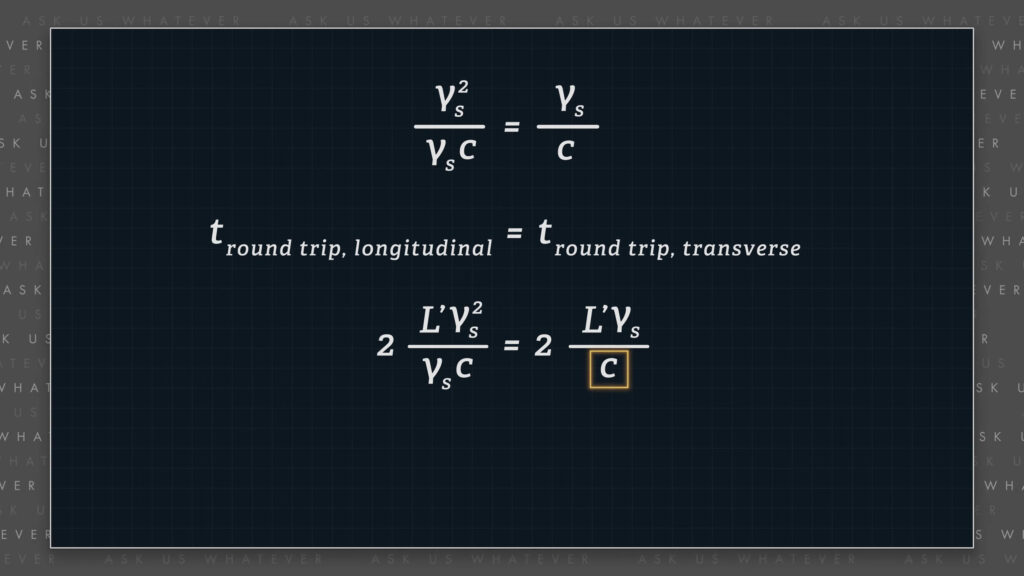
\(\frac{\gamma^2_s}{\gamma_s c} = \frac{\gamma_s}{c} \)
So, the assumption that the time dilation factor \(\tau \), is equal to \(\gamma_s \), leads us to the conclusion that \(c_x \) equals \(\gamma_s \) times \(c \).
\(c_x = \gamma_s c \)
In which case our round trip travel times in both the longitudinal and transverse directions become equal.
\(t_{round \space trip} = 2\frac{L’\gamma^2_s}{\gamma_s c} = 2\frac{L’\gamma_s}{c} \)
Two times the longitudinal path length \(L’ \) times \(\gamma_s \) squared, divided by \(x \)-direction light speed, \(\gamma_s \) times \(c \), is equal to two times the transverse path length \(L’ \) times \(\gamma_s \) divided by \(c \).
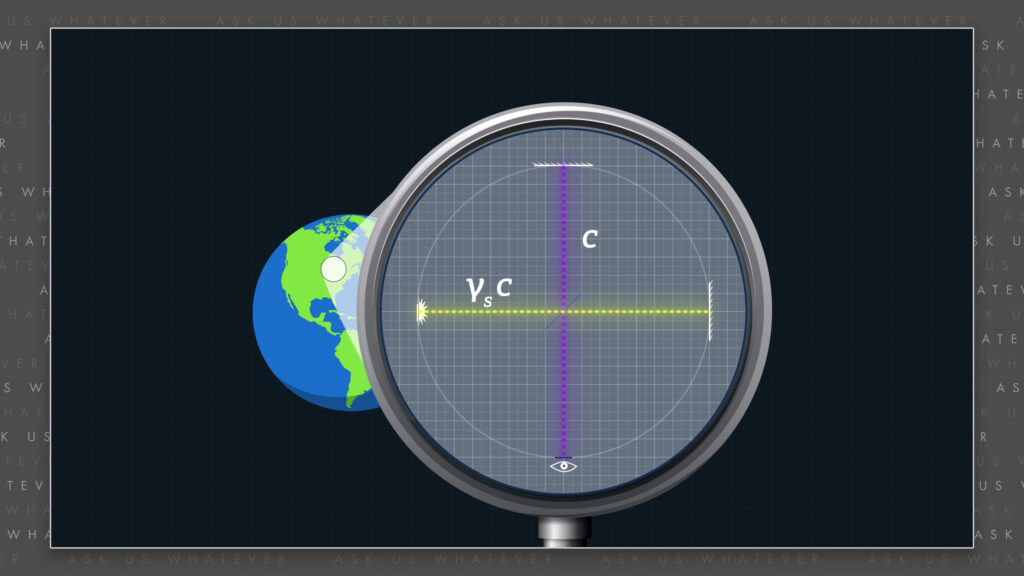
In plain English, if light travels at speed \(\gamma_s \) times \(c \) in the longitudinal direction, and travels at speed \(c \) in the transverse direction, then light will travel along perpendicular light paths in exactly the same amount of time regardless of the speed of the inertial reference frame in which those light paths are located. We have potentially solved the Michelson Morley mystery without invoking length contraction!
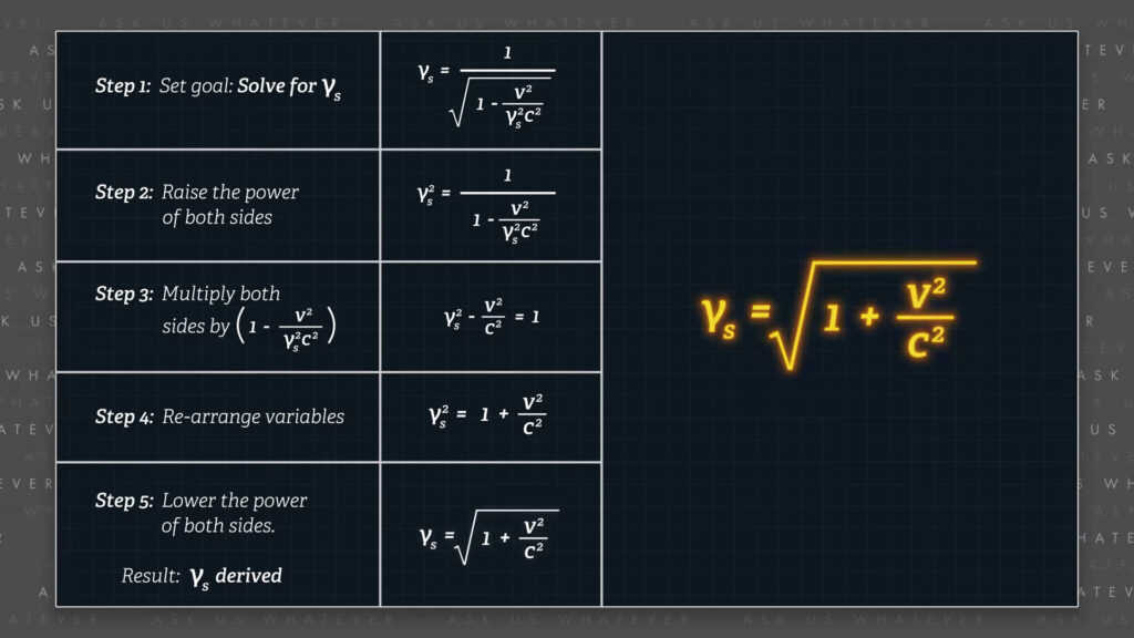
So, if our assumption about time-dilation is correct, what’s the formula for \(\gamma_s \)? We can derive it by rewriting the modified Lorentz formula with \(\gamma_s \) times \(c \) instead of \(c_x \),
\(\gamma_s = \frac{1}{\sqrt{1-\frac{v^2}{c^2_x}}} = \frac{1}{\sqrt{1-\frac{v^2}{\gamma^2_s c^2}}} \)
and then solving for \(\gamma_s \) doing some fast algebra. You can pause the screen here if you want to study it closely.
\(\gamma^2_s = \frac{1}{1-\frac{v^2}{\gamma^2_s c^2}} \)
\(\gamma^2_s – \frac{v^2}{c^2} = 1 \)
\(\gamma^2_s = 1 + \frac{v^2}{c^2} \)
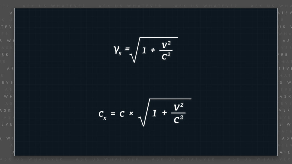
\(\gamma_s = \sqrt{1+\frac{v^2}{c^2}} \)
We find that \(\gamma_s \) equals the square root of one plus \(v \) squared divided by \(c \) squared.
And so longitudinal light speed, as measured from the stationary frame when light is emitted from a moving source, is equal to,
\(\text{longitudinal light speed} = \)
\(c \sqrt{1+\frac{v^2}{c^2}} \)
And so longitudinal light speed, as measured from the stationary frame when light is emitted from a moving source, is equal to,
\(\text{longitudinal light speed} = \)
\(c \sqrt{1+\frac{v^2}{c^2}} \)
\(c \) times the square root of 1 plus \(v \)-squared over \(c \)-squared.
Now, skeptics are going to question the concept of variable light speed. And so I want to make a few things clear up front. First of all, the transformations we’ll derive in the next episode will show that light will always be observed to travel at speed \(c \), in all directions, when coming from a stationary source within any given inertial reference frame – like the Earth. Only those observers who witness light coming from a moving source will be able to detect it traveling faster than \(c \). And the source will have to be traveling extremely fast in order to notice the difference.
The numerical values of \(\gamma_s \) and the Lorentz \(\gamma \) factor are almost identical at the typical travel speeds of planets and GPS satellites. The degree of time dilation due to motion as experienced by GPS satellites would be numerically identical down to 15 digits when computed with either \(\gamma_s \) or the Lorentz \(\gamma \) formula. In other words, these \(\gamma \) factors are indistinguishable at source speeds we’ve been able to measure (and I just want to say up front, that there is a caveat for particles accelerated by a field that, itself, operates at speed \(c \) in the stationary frame, like an electric or magnetic field. But that’s going to be taken up in a whole new episode.).
Waves generally travel at a speed determined by a medium that accommodates their movement. When we consider sound waves or water waves, the medium has mass. So the waves have to displace that mass in order to propagate, which affects the speed at which the waves can travel.

But light waves are different. Einstein didn’t believe in an ether. So whether there is no ether, or perhaps an ether without mass, then mass does not factor into the propagation speed of light waves. In other words, there is no a priori reason why light waves could not travel at different speeds in different directions, given that they are not required to displace a massive medium. And so it’s possible for light waves to travel at speed \(\gamma_s \) times \(c \) in the longitudinal direction and at speed \(c \) in the transverse direction.
We’ll spend much more time with \(\gamma_s \) in the future. But I’d like to tease you with a few observations: \(\gamma_s \) does not have a singularity. When \(v \) equals \(c \), \(\gamma_s \) is simply \(\sqrt{2} \), instead of infinity. One of the reasons why Einstein assumed that nothing can travel faster than speed \(c \), is that the Lorentz \(\gamma \) factor blows up to infinity when \(v \) equals \(c \). Not so for \(\gamma_s \). Matter and/or energy can, in theory, travel faster than speed \(c \) under the alternative model.
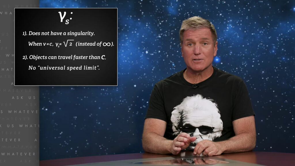
The possibility of superluminal motion provides a potential answer to the size of the universe. It has been estimated that the universe is about 100 billion light years in diameter. Whereas the age of the universe has been estimated to be roughly 14 billion light years, which would limit its diameter to 28 billion light years if nothing can travel faster than \(c \).
The alternative model, and its formula for \(\gamma_s \) provides an answer to that dilemma. It allows for objects in our universe to travel at speeds faster than \(c \), without having to postulate a fanciful stretching of space-time. I hope the possibility of superliminal travel is starting to intrigue you.
Alright, we’re going to end this video here and continue with the derivation of the alternative model in the next episode. If you have any questions, please write them in the comments section. I’m Joe Sorge, and thanks for watching.