Hey, welcome to Ask Us Whatever. I’m Joe Sorge.
Alright, in Episode 7.1 you heard me pick apart the Lorentz transformations, because I believe they were derived with some questionable assumptions. And then in Episode 7.2, we reviewed Einstein clock synchronization.
So, now that we’ve laid some groundwork, we’re going to derive the time and distance transformations for the Alternative Model, and show that they provide solutions to many of the weaknesses inherent in the Lorentz transformations and in Special Relativity.
And if you have not watched Episode 7.1, you may want to, because we are going to rely on some of the same nomenclature and concepts introduced there.
Okay, to derive the Alternative Model transformations, we will piggyback on the derivation of the longitudinal Lorentz transformations up to the point where capital \(C \) equals some type of time dilation factor, which we will call gamma for now, and that capital \(B \) equals capital \(C \) times \(v \). That gets us to these generic formulas for Lorentz-style transformations.
\(dx=Adx^{\prime} + \gamma v dt^{\prime} \)
\(dt=Ddx^{\prime}+\gamma dt^{\prime} \)
\(dx^{\prime}= \frac{(dx-vdt)}{(A-vD)} \)
\(dt^{\prime}=\frac{(Adt-Ddx)}{\gamma(A-vD)} \)
So, when \(dt \) is zero, the \(dx^{\prime} \) reverse transformation becomes,
\((dt=0) \hspace{2cm} dx^{\prime} = \frac{dx}{(A-vD)} \)
\(dx \) divided by \(A \) minus \(v \) times \(D \). Note that I called it a reverse transformation, not an inverse transformation. I am not making any assumptions about symmetry between the primed and unprimed transformations.
Now, when dt equals zero \((dt=0) \), such that events are simultaneous in the stationary frame, the distance between the same events in the moving frame will be related to the distance in the stationary frame
\((dt=0) \hspace{2cm} dx^{\prime} = \frac{dx}{(A-vD)} \)
by a factor of \(A \) minus \(v \) times \(D \). If lengths do not contract in the real world (and as I’ve said, the concept of length contraction was conjured up by Lorentz and Einstein when they couldn’t figure out any other way to explain the Michelson Morley result) the distance \(dx^{\prime} \) simply equals \(dx \); and therefore, A minus v times D must equal 1.
\(A-vD=1 \)
We need to solve for capital \(A \) and capital \(D \). Let’s look at conditions where \(dx \) equals zero \((dx=0) \), such that the \(dx \) transformation becomes, capital A times \(dx^{\prime} \) plus gamma times \(v \) times \(dt^{\prime} \) equals zero. This can be rearranged to solve for \(\frac{dx^{\prime}}{dt^{\prime} }\), which equals negative gamma times \(v \) divided by \(A\).
\(dx=Adx^{\prime}+\gamma vdt^{\prime}=0 \)
\( \frac{dx^{\prime}}{dt^{\prime}}=\frac{-\gamma v}{A}\)
Now recall from Episode 7.1 that this is where the Lorentzians make the assumption that \(\frac{ dx^{\prime} }{dt^{\prime} } \) must equal negative v, without addressing the concern that \(\frac{ dx^{\prime} }{dt^{\prime} } \) is measured in meters per second\(^{\prime} \) and \(v \) is measured in meters per second. Their approach requires capital \(A \) to be a dimensionless conversion factor, relating distance traveled between the two frames, which in the classical world would be a function of gamma squared, not gamma. Their conclusion that capital \(A \) must equal gamma cannot be arrived at using this formula alone.
The Lorentzians must also invoke their assumption about distance conversion, namely they must invoke the assumption that lengths contract in order to deem capital \(A \) to be equal to gamma \((A=\gamma) \) .
And since our goal is to see if we can derive the most general form of transformation, without making a priori assumptions about light speed or length contractions, let’s pursue a different approach to deriving the value of capital \(A \).
Recall from Episodes 2 and 6 that \(dx_{average} \) can be obtained for a longitudinal signal when that signal travels to the front of a non-contracting, moving train car and bounces back to the rear of the train car, using the formula,
\(dx_{average} = \frac{1}{2} (\frac{dx^{\prime}}{c_x-v}+\frac{dx^{\prime}}{c_x+v}) c_x \)
\(dx_{average} = \frac{1}{1-\frac{v^2}{c_x^2 }} dx^{\prime} \)
\(dx^{\prime} \) multiplied by the square of a Lorentz-type gamma factor, where the speed of longitudinal signal is represented by the symbol \(c_x \), (which is a symbol we use so that we can retain the possibility that longitudinal light speed might not simply be speed \(c \)).
As we described in Episode 6, we use the symbol \(\gamma_s^2 \) to represent this Lorentz-type gamma factor squared.
\(\frac{1}{1-\frac{v^2}{c_x^2 }} dx^{\prime} = \gamma_s^2 dx^{\prime} \)
And since \(dx_{average} \) is equal to one half the sum of the forward and reverse distance transformations,
\(dx_{average}=\frac{1}{2} (Adx^{\prime} + \gamma vdt^{\prime} + Adx^{\prime}-\gamma vdt^{\prime} ) = Adx^{\prime} \)
then,
\(Adx^{\prime}=\gamma_s^2 dx^{\prime} \)
capital A times \(dx^{\prime} \) equals \(\gamma_s^2 \) times \(dx^{\prime} \).
So, we can logically conclude that capital A equals \(\gamma_s^2 \).
\(A=\gamma_s^2 \)
And therefore, let’s update our transformations by substituting \(\gamma_s^2 \) for \(A \).
\(dx=\gamma_s^2 dx^{\prime}+\gamma_s vdt^{\prime} \)
\(dt=Ddx^{\prime}+\gamma_s dt^{\prime} \)
\(dx^{\prime}=\frac{dx-vdt}{\gamma_s^2-vD} \)
\(dt^{\prime}=\frac{\gamma_s^2 dt-Ddx}{\gamma_s (\gamma_s^2-vD) } \)
We now only need to find capital \(D \) and we’re finished!
Recall from the \(dx^{\prime} \) reverse transformation that capital \(A \) minus \(v \) times capital \(D \) equals 1.
\(A-vD=1 \)
And since capital \(A \) is equal to \(\gamma_s^2 \), then \(\gamma_s^2 \) equals 1 plus \(v \) times capital \(D \).
\(\gamma_s^2=1+vD \)
Recall from Episode 6.1 that gamma-s is equal to, the square root of 1 plus \(v \)-squared over \(c \)-squared.
\(\gamma_s = \sqrt{\frac{1}{1-\frac{v^2}{c_x^2} }} = \sqrt{\frac{1+v^2}{c^2 }} \)
Which means that, capital \(D \) equals \(v \) divided by \(c^2 \).
\(D=\frac{v}{c^2} \)
This means that the Alternative Model clock-offset term differs from the Lorentz clock offset term by a factor of gamma.
Lorentz clock offset term = \(\frac{\huge{\gamma}\normalsize{v}}{c^2 } dx^{\prime} \)
Alternative clock offset term = \(\frac{v}{c^2 } dx^{\prime} \)
So, we can now write our alternative to the Lorentz transformations by substituting the values for \(A \), \(B \), \(C \) and \(D \) into the general formulas.
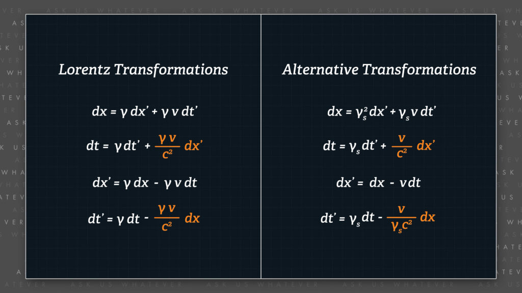
Alternative Time and Distance Transformations
\(dx=\gamma_s^2 dx^{\prime}+\gamma_s vdt^{\prime} \)
\(dt=\gamma_s dt^{\prime}+\frac{v}{c^2} dx^{\prime} \)
\(dx^{\prime}= \frac{dx-v dt}{1} \)
\(dt^{\prime}=\gamma_s dt- \frac{v }{\gamma_s c^2 } dx \)
These transformations describe the real-world relationship between frames S and S\(^\prime \). They are a bit more complex than the Galilean transformations, but still grounded in reality. They do not resort to length contraction, or the stretching of spacetime, or the superposition of clocks beating at two different rates at the same time. They just follow some basic rules of physics.
Now when we introduced the possibility of variable light speed in Episode 6, a number of critics raised their swords in anger. Well, I want to show you something magical about the alternative transformations. Let’s compute the speed of light in the S\(^\prime \) frame, \(\frac{dx^{\prime} }{dt^{\prime}} \), by taking the ratio of the two transformations.
\(\frac {dx^{\prime}}{dt^{\prime} } = \frac{dx-vdt}{\gamma_s dt-\frac{vdx}{\gamma_s c^2 }} \)
\(\frac{dx^{\prime}}{dt^{\prime}} = \frac{\frac{dx-vdt}{\gamma_s dt}}{\frac{\gamma_s dt}{\gamma_s dt}-\frac{v}{\gamma_s c^2 }\times \frac{dx}{\gamma_s dt}} \)
Let’s divide the top and bottom of the right-hand ratio by gamma-s times \(dt \),
\(\frac{dx^{\prime}}{dt^{\prime}} = \frac{\frac{dx}{\gamma_s dt} – \frac{v}{\gamma_s}} {1-\frac{v}{\gamma_s c^2} \times \frac{dx}{\gamma_s dt}} \)
And then substitute our speed of light, as seen from the stationary frame, \(\gamma_s \) times \(c \), for \(\frac{dx}{dt} \).
\(\frac{dx}{dt} = \gamma_s c \)
\(\frac{dx^{\prime}}{dt^{\prime}} = \frac{ \frac{ \gamma_s c}{\gamma_s} – \frac{v}{\gamma_s} }{ 1 – \frac{v}{\gamma_s c^2} \times \frac{\gamma_s c}{\gamma_s} } \)
You can pause the video to check the fast algebra.
\(\frac{dx^{\prime}}{dt^{\prime}} = \frac{c-\frac{v}{\gamma_s}}{1- \frac{v}{\gamma_s c}} \)
\(\frac{dx^{\prime}}{dt^{\prime}} = c \frac{1-\frac{v}{\gamma_s c}}{1- \frac{v}{\gamma_s c}} \)
\(\frac{dx^{\prime}}{dt^{\prime}} = c \frac{meters}{second^\prime} \)
Even if the speed of light as observed from the stationary frame is not \(c \), the speed of light measured in the S’ frame is \(c \) meters per second\(^\prime \), just like in special relativity. Why? Because the Alternative Model also uses Einstein synchronization to adjust its clocks in a manner that is similar to how it’s done in Special Relativity. And as I pointed out in Episode 7.2, light appears to travel at a constant speed in all inertial reference frames if the clocks are synchronized using the protocol Einstein described in his 1905 paper on relativity.
That protocol leads to clocks that exhibit different readings depending on their location along the axis of motion. Without such a synchronization protocol, light would appear to travel at different speeds when traveling parallel versus antiparallel to the axis of reference frame motion. We’ve incorporated Einstein’s synchronization protocol into the Alternative Model for ease of comparison to Special Relativity. But we could elect to work with absolutely synchronized clocks as well, by changing the distance and time transformations accordingly.
We will show in a future episode that the speed of light in the y and z directions is \(c \) as well. That is, in the Alternative Model, electromagnetic radiation is observed to travel at speed \(c \) in all directions within all inertial reference frames, regardless of the speed of the reference frame. Thus, any physics formulas that use a constant c for the observed speed of light in all inertial frames will be the same for the Alternative Model as they are for Special Relativity. So those of you who point to Maxwell’s equations as validation of the Special Theory of Relativity, well you are also going to have to acknowledge that the same argument supports the Alternative Model as well.
By the way, I think that the Maxwell equation argument might be fallacious for both models, because light speed is only constant if one adjusts the clocks used to measure light speed according to Einstein’s synchronization protocol, which deploys circular logic to force light to travel at speed \(c \).
I don’t think electrical circuits care about clocks, so this raises the question of whether electrical and magnetic fields would change under relativistic conditions, or is the \(c \) term in Maxwell’s equations a simple unit conversion constant, such as the speed of light when emitted by a source that is stationary within the universal, preferred reference frame. Or is it a representation of light speed within any inertial frame? It’s worth thinking about.
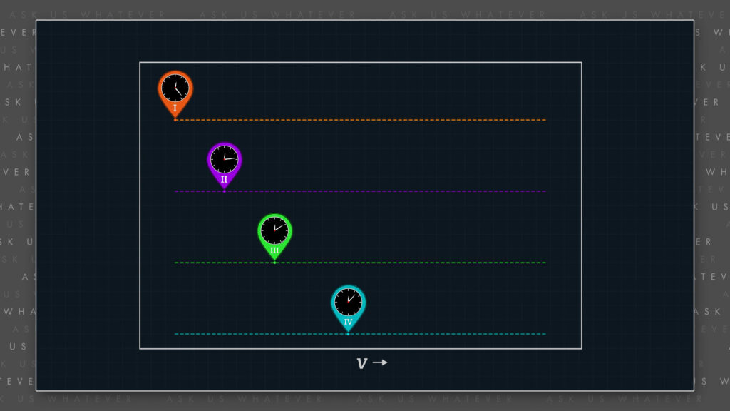
Before we conclude I’d like to point out that in the Episode 7.1 we criticized the Lorentz transformations because they require the clocks in each reference frame to be Einstein-synchronized with respect to the speed of an arbitrary reference frame. And this created an impossible conflict when the clocks in a first frame needed to be Einstein synchronized relative to two other reference frames each moving at different speeds.

So, I’m anticipating that the skeptics in this audience will ask why the Alternative Model doesn’t suffer from the same criticism. I mean after all, the alternative transformations also include clock offset terms.
Well, the answer is that the clocks in the Alternative Model are all synchronized relative to a single, preferred reference frame. Do you recall the master of the universe eating Cheetos in the cosmic train station in Episode 3.2?
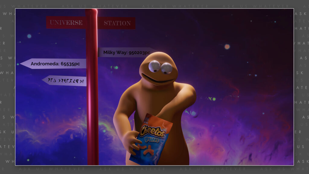
Well, if the cosmic train station is truly stationary within a universal preferred reference frame, then the speed of the cosmic train station relative to itself, \(v \), is zero. Which means that the clock offset term in the alternative dt transformation for the universal, preferred reference frame is also zero.
\(\frac{v}{c^2} dx^{\prime}= \frac{0}{c^2} dx^{\prime}=0 \)
In other words, if we were to synchronize the clocks in the preferred reference frame, we would set them all to the same time value. This is true in Special Relativity as well, but most physicists have grossly misinterpreted Einstein’s 1905 paper and have attributed a non-existent symmetry to Special Relativity based on the inverse Lorentz transformations, which I believe are erroneous. The inverse Lorentz \(dt^{\prime} \) transformation is a mathematical convenience, but it has no meaning in the real world. And so, I prefer an alternative format for the reverse \(dt^{\prime} \) transformation in the Alternative Model.
Let’s rewrite the \(dt^{\prime} \) transformation, by rearranging the \(dt \) transformation to solve for \(dt^{\prime} \).
\(dt=\gamma_s dt^{\prime} + \frac{v}{c^2} dx^{\prime} \)
\(\gamma_s dt^{\prime}=dt-\frac{v}{c^2} dx^{\prime} \)
\(dt^{\prime} = \frac{dt}{\gamma_s} -\frac{v}{\gamma_s c^2} dx^{\prime} \)
A couple of algebraic steps shows us that \(dt^{\prime} \) can be set equal to \(dt \) divided by \(\gamma_s \) minus \(v \) times \(dx^{\prime} \) divided by \(\gamma_s \) times \(c^2 \). In other words, time in the S\({^\prime} \) frame, \(dt^{\prime} \), is equal to time in the S frame, dt divided by the time dilation factor \(\gamma_s \), as further adjusted for the effects of the Einstein synchronization protocol on the clocks
in the S\(^{\prime} \) frame.
\(\frac{v}{\gamma_s c^2} dx^{\prime}\)
That adjustment is equal to the speed of the S\(^{\prime} \) frame, \(v \), relative to the universal, preferred frame, times the physical separation of any two given clocks in the S\(^{\prime} \) frame, \(dx^{\prime} \), divided by \(\gamma_s \) times \(c^2 \). In the next episode I’ll show you how we can determine \(v \) relative to the universal, preferred frame by measuring the clock offset.
If we compare the \(dx^{\prime} \) term here to the \(dx^{\prime} \) term in the dt transformation,
\(\frac{-v}{\gamma_s c^2} dx^{\prime} \text{ vs } \frac{v}{c^2} dx^{\prime} \)
we see that the clock offset term of the \(dt^{\prime} \) transformation is the same as the clock offset term for the \(dt \) transformation except that the former contains a \(\gamma_s \) term in the denominator, and is of opposite sign.
\(dt^{\prime} = \frac{dt}{\gamma_s} -\frac{v}{\gamma_s c^2}dx^{\prime} \)
\(dt=\gamma_s dt^{\prime} + \frac{v}{c^2} dx^{\prime} \)
In other words, the \(dt^{\prime} \) and \(dt \) transformations take their offset readings only from the clocks in the S\(^{\prime} \) reference frame, and then express the time difference either in units of seconds\(^{\prime} \) for the \(dt^{\prime} \) transformation, or in units of seconds for the \(dt \) transformation.
Einstein synchronization causes time, in units of seconds\(^{\prime} \), to be subtracted from clocks in the S\(^{\prime} \) frame that lie in the positive direction along the axis of motion. Whereas the \(dt \) transformation must add that time back, in units of seconds, to produce an array of clocks that all report the same readings regardless of their position along the corresponding axis in frame S.
In other words, these two clock offset terms describe the time readings of same clocks in frame S\(^{\prime} \), merely stated in terms of seconds\(^{\prime} \) or seconds to properly suit the units being used in the corresponding transformation.
\(dx^{\prime} \) term of new \(dt^{\prime} \) transformation \(= \)
\(\frac{v}{\gamma_s c^2} dx^{\prime}\) (seconds\(^{\prime} \))
\(dx^{\prime}\) term of \(dt \) transformation =
\(\frac{v}{c^2} dx^{\prime} \) (seconds)
Thus, by adopting the concept of a universal preferred reference frame and by eliminating the fantasy of length contraction, the Alternative Model brings relativity back into the realm of reality and gives us the tools to begin to understand our universe without the need to invoke fantastical workarounds like worm holes and magical clocks and the stretching of spacetime. Such fantasies might be the fun concepts for Hollywood movies, but serious physicists should now think long and hard about invoking them to explain the world we live in.
Alright! That’s it for now. If you have any questions, please write them in the comments section. I’m Joe Sorge, and thanks for watching.